LEN Function Examples – Excel, VBA, & Google Sheets
Written by
Reviewed by
Download the example workbook
This tutorial demonstrates how to use the LEN Function in Excel to count the number of characters.
What Is the LEN Function?
The Excel LEN Function (Len is short for “length”), tells you the number of characters in a given text string.
Although it is mainly used for string (text) data, you can also use it on numerical data – but as we’ll see, there are a few things you need to keep in mind.
How to Use the LEN Function
To use the Excel LEN Function, type the following, putting any text string, cell reference, or formula between the parentheses:
=LEN(B2)Let’s take a look at some examples:
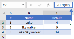
In example #1, we’ve asked LEN how many characters are in cell B2, which contains “Luke” – so Excel returns 4.
Combine the LEN Function
If you want to return the total number of characters in two cells, you have a couple of options. You can either concatenate the two cells using an ampersand (“&”) as in example #1, or you can use LEN on both cells and sum the results, as in example #2.
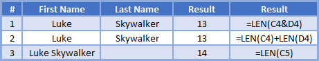
Important note: LEN counts spaces as characters. Look at example #3 – in this case, LEN returns 14 because it’s also counting the space between “Luke” and “Skywalker”.
How LEN Handles Numbers
The LEN Function is designed to return the number of characters in a text string. If you pass a number, LEN first converts it to a string, and then returns its length.
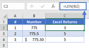
As you can see, LEN counts decimal points, and if you format a cell to a currency, the currency symbol is not counted.
How LEN Handles Formatted Cells
Have a look at the following examples:
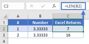
Cells B2 and B3 both contain the same figure: 3.33333. So why does LEN return different values for each?
The answer is that in B2 I typed the value 3.33333, but in B3 I typed the formula =10/3, and then formatted it to 6 decimal places.
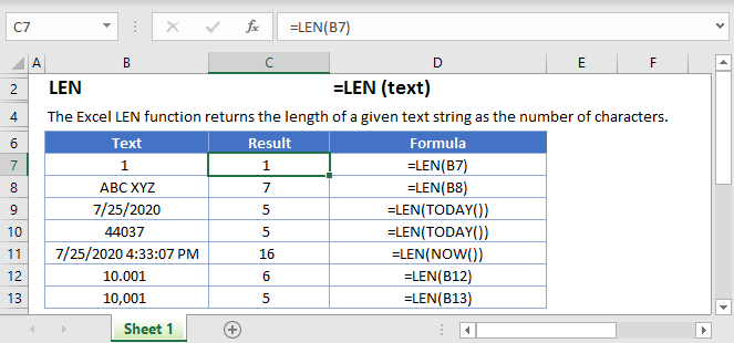
With formatted cells, LEN returns the actual value of the cell, regardless of the number of decimal places you’ve chosen to display.
But why 16? That’s because Excel can store a maximum of 15 numbers in a cell, and will clip longer numbers once they reach this limit. So LEN returns 16: 15 numbers, plus the decimal point.
How LEN Handles Dates
Excel stores dates as numbers, represented as the number of days since January 0, 1900.
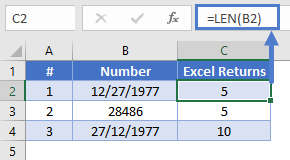
Examples #1 and #2 are equivalent, it’s just that B2 is formatted as a date, and B3 as a number. So LEN returns 5 either way.
Example #3 is formatted as text, so LEN returns 10. This is the same as typing =LEN(“27/12/1977”).
Useful LEN examples
You can combine LEN with some of the Excel functions in some useful ways.
Trimming a Given Number of Characters from the End of a String
You can combine LEN with LEFT to trim a given number of characters from the end of a string. If the string you want to trim was in A2, and you wanted to trim 5 characters from the end, you’d do it like this:
=LEFT(A2, LEN(A2)-5)The LEFT Excel Function returns a given number of characters from the beginning of a string.
Check out the example below:
=LEFT(A2, LEN(A2)-5)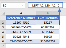
Here we have a series of reference numbers with a four-digit area code on the end. We’ve used LEN with LEFT to take the strings in column A, and return a number of characters equal to the length of the string, minus 5, which will get rid of the four digits and the hyphen.
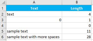
Using LEN Without Counting Leading and Trailing Whitespace
Sometimes our cells might contain spaces before and after the actual data itself. This is common when data is manually entered, and sometimes people accidentally pick up a space when copying and pasting data.
This can throw off our LEN function results, but we can solve that problem by combining LEN with TRIM, like so:
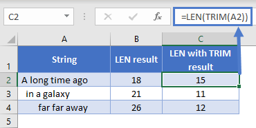
=LEN(TRIM(A2))TRIM removes any trailing or leading spaces from a string. In the example below, each sentence has spaces either before or after the text. Note the different results between LEN and LEN with TRIM.
Using LEN with SUBSTITUTE to Avoid Counting a Given Character
If you want to count the number of characters in a string, but you don’t want Excel to count a particular character, you can do this by combining LEN with SUBSTITUTE.
With SUBSTITUTE, you can take a string, and swap any character or substring within it for anything else. We can use SUBSTITUTE to replace the character we don’t want to count with nothing, effectively removing it.
For example:
=SUBSTITUTE("Han Solo", " ", "")Will return:
HanSolo
So, imagine we have a list of names, and we want to know the number of characters in each name. However, the first and last names are stored in the same cell, and we don’t want to count the space between them.
We could combine LEN with SUBSTITUTE as follows:
=LEN(SUBSTITUTE(A2," ", ""))Which would give us the following results:
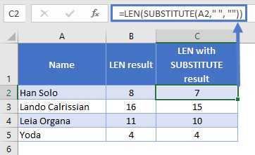
Note that as the fourth example has no spaces, both formulas produce the same result.
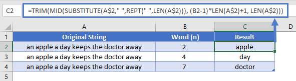
Find Nth word in the String
We could combine TRIM, MID, SUBSTITUTE, REPT with LEN as follows to get last word of the string.
=TRIM(MID(SUBSTITUTE(A$2," ",REPT(" ",LEN(A$2))), (B2-1)*LEN(A$2)+1, LEN(A$2)))Which would give us the following results:
Extract Number from the Left/Right of a string
When you working with excel you need to exact the number from given detail. Sometime you need to exact number from Left and sometime you need to extract number from Right. So LEN function will help you to do this task by combining with few other functions.
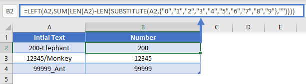
Extract Number from the Left
We could combine LEFT, SUM, SUBSTITUTE with LEN as follows:
=LEFT(A2,SUM(LEN(A2)-LEN(SUBSTITUTE(A2,{"0","1","2","3","4","5","6","7","8","9"},""))))Which would give us the following results:
Extract number from the Right
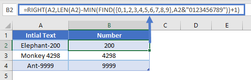
We could combine RIGHT, MIN, FIND with LEN as follows:
=RIGHT(A2,LEN(A2)-MIN(FIND({0,1,2,3,4,5,6,7,8,9},A2&"0123456789"))+1)Which would give us the following results:
LEN with REPT to add leading ZEROS to Number
Add leading ZEROS is very useful when you working with excel. In this example we will explain how you can do this by combining LEN with REPT.
=REPT(0, 6-LEN(A2))&A2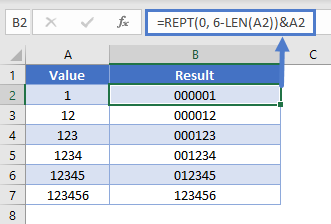
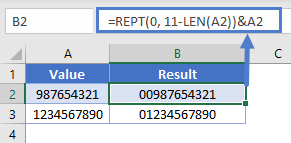
In above example we explain add leading zeros only till 5 digits, but based on the requirement you can change number 6 to get required out put. you can refer below example to get leading zero up to 10 digits.
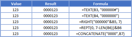
More Examples for Add leading ZEROS to number.
Below table help you give more ways for add leading zeros to set number.
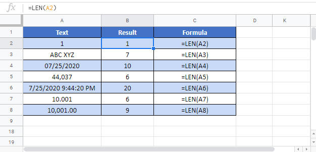
LEN in Google Sheets
The LEN Function works exactly the same in Google Sheets as in Excel:
LEN Examples in VBA
You can also use the LEN function in VBA. Type:
application.worksheetfunction.len(text)Executing the following VBA statements
Range("B2") = Len(Range("A2"))
Range("B3") = Len(Range("A3"))
Range("B4") = Len(Range("A4"))
Range("B5") = Len(Range("A5"))
Range("B6") = Len(Range("A6"))
will produce the following results