SUMIF, COUNTIF, and AVERAGEIF Functions – The Master Guide
Written by
Reviewed by
This Excel Tutorial demonstrates how to use the Excel Countif and Countifs Functions.
Formula Examples:

COUNTIF Function Description:
Counts all cells in a series that meet one (COUNTIF) or multiple (COUNTIFS) specified criteria.
COUNTIF Syntax
range – An array of numbers, text, or blank values.
criteria – A string containing the criteria. Example “>0”
More Examples:
First let’s look at an easy COUNTIF example:
COUNTIF Greater than Zero
This code will count all cells that are greater than zero in column A.
=countif(a4:a10,">0")COUNTIF Less Than Zero
This code will count all cells that are less than zero in column A.
=countif(a4:a10,"<0")COUNTIF Blank Cells
=countif(a4:a10,"")This COUNTIF formula counts all the blank cells in column A. However, instead, you could use COUNTBLANK to count all the blank cells:
=countblank(a4:a10)Count Not Blank Cells
Counting nonblank cells is a little trickier. You would think that this would count all the non-blank cells:
=countif(a4:a10,"<>")and it usually does, except for one notable exception. When a cell contains a formula that results in “” (Blank), the above code will count it as non-blank because a formula exists in the cell. Instead, use this formula:
=countif(a4:a10,"*?")This formula makes use of Wildcard Characters. We’ll learn about them below.
There is one other count function you should know: the COUNTA Function. The COUNTA Function counts all cells that contain anything: a formula (even if it results in “”), a logical value (TRUE or FALSE), text, or a number.
Count Blank and Non-Blank Cell Examples:
!!!!!!!!!picture of the various examples!!!!!!!!!!
(mention counta?)
Countif Wildcard
You may have heard about Wildcards in Excel. Wildcards are characters that can represent any character. Here’s a chart:
<>
picture with apples
Text – Exact Match
=countif(a2:a10,"apples")Text – Contains Text
=countif(a2:a10,"*apples*")Text – Contains Any Text
=countif(a2:a10,"*")Countif – Does not Contain any Text
=countif(a2:a10,"<>*")Countif Color
Unfortunately there is not an easy way to count cells with specific colors. To do this you will need to use VBA. Here’s a link with more information: CountIf Cell Color using VBA>.
Countif Duplicates
There are numerous ways to count duplicates, but let’s take a look at one of the easier methods, using only COUNTIF functions.
Picture
First, create a column to count how often a record appears on the data. Any record appearing more than once (>1) is considered a duplicate.
=countThen we create a COUNTIF function to count the number of records that appear more than once:
=countCountif with Two or Multiple Conditions – The Countifs Function
So far we’ve worked only with the COUNTIF Function. The COUNTIF Function can only handle one criteria at a time. To COUNTIF with multiple criteria you need to use the COUNTIFS Function. COUNTIFS behaves exactly like COUNTIF. You just add extra criteria. Let’s take a look at some examples…
IMAGE
COUNTIFS – Greater Than and Less Than
Let’s do a COUNTIF where we check if a number falls within a range. The number must be greater than 0, but less than 100:
COUNTIFS – Date Range
Now let’s try it with dates. Find any dates within the range 1/1/2015 to 7/15/2015:
COUNTIFS – Or
So far we’ve only dealt with AND criteria. Ex: Greater than 0 AND less than 100. What doing a COUNTIFS with OR?
countif pivot table
How to do a Countif in Excel
Criteria for Countif
have hyperlinks at the top to the various sections
have links to his content on the formula page with # to link to different stuff
when you apply criteria treat it like text
image
Syntax and Arguments:
x –
COUNTIF VBA Examples
You can also access the Excel COUNTIF Function from within VBA, using Application.WorksheetFunction.
Type:
application.worksheetfunction.CountIf(Range, Criteria)
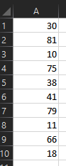
Assuming we have the data displayed above:
WorksheetFunction.CountIf(Range("A1:A10"), ">60")Will return 4 , as there are four cells with values larger that 60
WorksheetFunction.CountIf(Range("A1:A10"), "10")Will return 1 , as there is one cell with value equal to 10
MsgBox WorksheetFunction.CountIf(Range("A1:A10"), "<>")Will return 10 , as all cells have values
MsgBox WorksheetFunction.CountIf(Range("A1:A10"), "")Will return 10 , as there are no blank cells
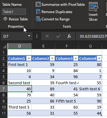
Assuming we have the data in a table named “Table1”, like displayed above:
WorksheetFunction.CountIf(Range("Table1"), "*test*")Will return 6, as there are six cells that contain the word “test”.
WorksheetFunction.CountIf(Range("Table1"), "test")Will return 6, as there are no cells that contain ONLY the word “test”.
WorksheetFunction.CountIf(Range("Table1"), "F*")Will return 6, as there are three cells whose values start with the letter “F”.
How to use the COUNTIF Function for Excel:
Return to the Function List
For more information about the COUNTIF Function visit the Microsoft COUNTIF help page.
Before we talk about how to use the countif function, we should mention these 3 other functions
count
counta
countblanks

