VBAガイド:ピボットテーブル編
In this Article
このチュートリアルでは、VBAを使用してピボットテーブルを操作する方法を説明します。
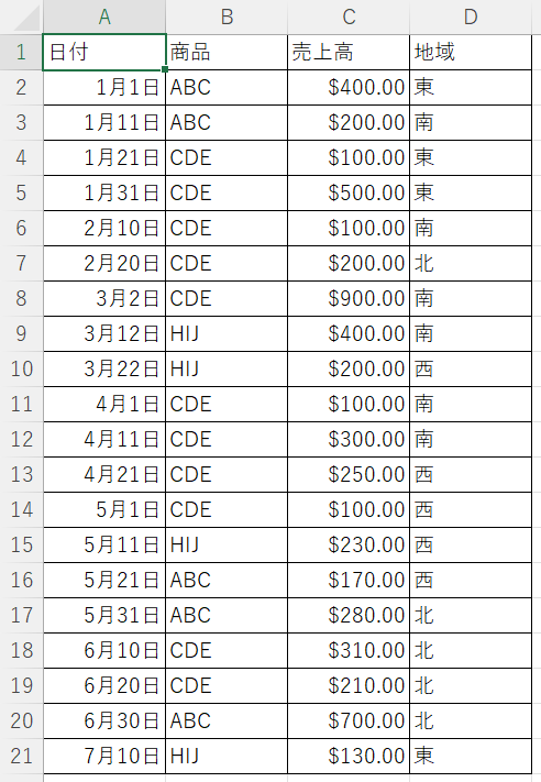
ピボットテーブルは、データから重要な洞察を引き出したり、要約したりするために使用できるデータ要約ツールです。例を見てみましょう。セル A1:D21 に、以下のような販売された製品の詳細を含むソース データセットがあります。
GetPivotDataを使用して値を取得する
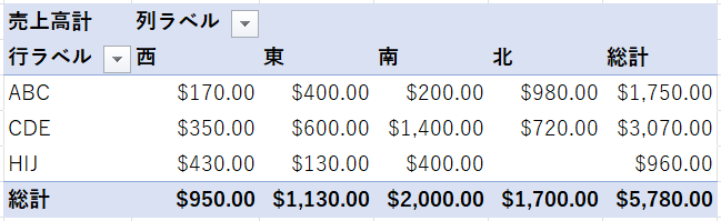
PivotTable1というピボットテーブルがあり、値/データフィールドが売上高、行フィールドが商品、列フィールドが地域であるとします。ピボットテーブルから値を返すには、PivotTable.GetPivotDataメソッドを使用することができます。 次のコードは、ピボットテーブルから1,130ドル(東地域の売上高合計)を返します。
MsgBox ActiveCell.PivotTable.GetPivotData("売上高", "地域", "東")
この場合、「売上高」がデータフィールド、フィールド1が「地域」、項目1が「東」です。 以下のコードでは、ピボットテーブルから980ドル(北地域の商品ABCの売上高合計)が返されます。
MsgBox ActiveCell.PivotTable.GetPivotData("売上高", "商品", "ABC", "地域", "北")この場合、売上高がデータフィールド、フィールド1が商品、項目1がABC、フィールド2が地域、項目2が北となります。 また、2つ以上のフィールドを含めることもできます。
GetPivotDataの構文は以下の通りです。
GetPivotData(データフィールド, フィールド1, 項目1, フィールド2, 項目2, …)
| パラメータ | 説明 |
|---|---|
| データフィールド | 売上、数量など、数字を含むデータフィールド |
| フィールド1 | テーブルの列または行のフィールド名 |
| 項目1 | フィールド1の項目名(オプション) |
| フィールド2 | テーブルの列または行のフィールド名(オプション) |
| 項目 2 | フィールド 2 の項目名(オプション) |
シート上でピボットテーブルを作成する
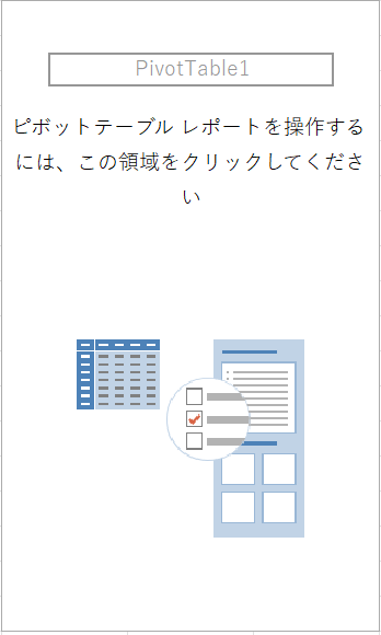
アクティブワークブックのSheet1のセルJ2に、上記のデータ範囲に基づいたピボットテーブルを作成するためには、以下のコードを使用します。
Worksheets("Sheet1").Cells(1, 1).Select

ActiveWorkbook.PivotCaches.Create(SourceType:=xlDatabase, SourceData:= _
  "Sheet1!R1C1:R21C4", Version:=xlPivotTableVersion15).CreatePivotTable _
  TableDestination:="Sheet1!R2C10", TableName:="PivotTable1", DefaultVersion _
  :=xlPivotTableVersion15

  Sheets("Sheet1").Select
結果は次のようになります。
新しいシートにピボットテーブルを作成する
アクティブなワークブックの新しいシートで、上記のデータ範囲に基づくピボットテーブルを作成するには、次のコードを使用します。
Worksheets("Sheet1").Cells(1, 1).Select

Sheets.Add
ActiveSheet.Name = "Sheet2"

    ActiveWorkbook.PivotCaches.Create(SourceType:=xlDatabase, SourceData:= _
  "Sheet1!R1C1:R21C4", Version:=xlPivotTableVersion15).CreatePivotTable _
  TableDestination:="Sheet2!R3C1", TableName:="PivotTable1", DefaultVersion _
  :=xlPivotTableVersion15

Sheets("Sheet2").Select
ピボットテーブルにフィールドを追加する
上記のデータ範囲を元に、新しく作成したPivotTable1というピボットテーブルにフィールドを追加することができます。注:ピボットテーブルを含むシートは、アクティブシートである必要があります。 行フィールドに商品を追加するには、次のコードを使用します。
ActiveSheet.PivotTables("PivotTable1").PivotFields("商品").Orientation=xlRowField

ActiveSheet.PivotTables("PivotTable1").PivotFields("商品").Position=1
列フィールドに地域を追加するには、以下のコードを使用します。
ActiveSheet.PivotTables("PivotTable1").PivotFields("地域").Orientation = xlColumnField

ActiveSheet.PivotTables("PivotTable1").PivotFields("地域").Position = 1
Value Sectionに商品を通貨単位の数値形式で追加するには、次のコードを使用します。
ActiveSheet.PivotTables("PivotTable1").AddDataField ActiveSheet.PivotTables( _
        "PivotTable1").PivotFields("売上高"), "売上高計", xlSum

    With ActiveSheet.PivotTables("PivotTable1").PivotFields("売上高計")

        .NumberFormat = "\$#,##0.00"

    End With
という結果になります。
ピボットテーブルのレポートレイアウトを変更する
ピボットテーブルのレポートレイアウトを変更することができます。以下のコードで、ピボットテーブルのレポートレイアウトをタブラーフォームに変更します。
ActiveSheet.PivotTables("PivotTable1").TableStyle2 = "PivotStyleLight18"ピボットテーブルを削除する
VBAを使用して、ピボットテーブルを削除することができます。以下のコードでは、アクティブシート上のPivotTable1というピボットテーブルを削除します。
ActiveSheet.PivotTables("PivotTable1").PivotSelect "", xlDataAndLabel, True
Selection.ClearContents
ワークブック内のすべてのピボットテーブルの書式設定
VBAを使用して、ワークブック内のすべてのピボットテーブルをフォーマットすることができます。次のコードは、ループ構造を使用して、ワークブックのすべてのシートをループし、ワークブック内のすべてのピボットテーブルをフォーマットします。
Sub FormattingAllThePivotTablesInAWorkbook()

Dim wks As Worksheet
Dim wb As Workbook
Set wb = ActiveWorkbook
Dim pt As PivotTable

For Each wks In wb.Sheets
  For Each pt In wks.PivotTables
    pt.TableStyle2 = "PivotStyleLight15"
  Next pt
Next wks

End SubVBAでのループの使い方については、こちらをご覧ください。
ピボットテーブルのフィールドを削除する
VBAを使用して、ピボットテーブルのフィールドを削除することができます。以下のコードは、アクティブシートのPivotTable1というピボットテーブルから、行セクションの商品フィールドを削除します。
ActiveSheet.PivotTables("PivotTable1").PivotFields("商品").Orientation = _
xlHidden
フィルタを作成する
PivotTable1というピボットテーブルが作成され、行セクションに商品、値セクションに売上高計が作成されています。ピボットテーブルには、VBAを使用してFilterを作成することもできます。以下のコードでは、フィルタセクションで地域を指定してフィルタを作成します。
ActiveSheet.PivotTables("PivotTable1").PivotFields("地域").Orientation = xlPageField

ActiveSheet.PivotTables("PivotTable1").PivotFields("地域").Position = 1
作成したフィルタに単一のレポート項目(ここでは東)を指定してピボットテーブルをフィルタするには、次のコードを使用します。
ActiveSheet.PivotTables("PivotTable1").PivotFields("地域").ClearAllFilters

ActiveSheet.PivotTables("PivotTable1").PivotFields("地域").CurrentPage = "東"
例えば、複数の地域(ここでは東と北)に基づいてピボットテーブルをフィルタしたい場合、次のようなコードになります。
ActiveSheet.PivotTables("PivotTable1").PivotFields("地域").Orientation = xlPageField

ActiveSheet.PivotTables("PivotTable1").PivotFields("地域").Position = 1

ActiveSheet.PivotTables("PivotTable1").PivotFields("地域"). _
EnableMultiplePageItems = True

With ActiveSheet.PivotTables("PivotTable1").PivotFields("地域")

.PivotItems("南").Visible = False

.PivotItems("西").Visible = False

End With
ピボットテーブルを更新する
VBAでピボットテーブルを更新することができます。VBAでPivotTable1という特定のテーブルを更新するには、次のコードを使用します。
ActiveSheet.PivotTables("PivotTable1").PivotCache.Refresh