Highlight Rows If (Conditional Formatting) – Excel & Google Sheets

This tutorial will demonstrate how to highlight rows if a condition in a cell is met using Conditional Formatting in Excel and Google Sheets.

 

 

Highlight Rows With Conditional Formatting

IF Function

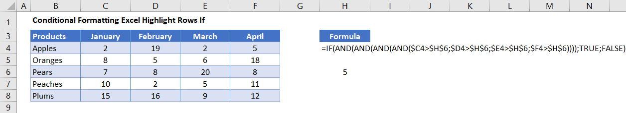
To highlight a row depending on the value contained in a cell in the row with conditional formatting, you can use the IF Function within a Conditional Formatting rule.

1. Select the range you want to apply formatting to.
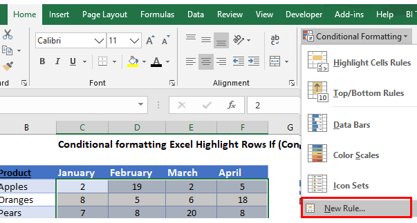
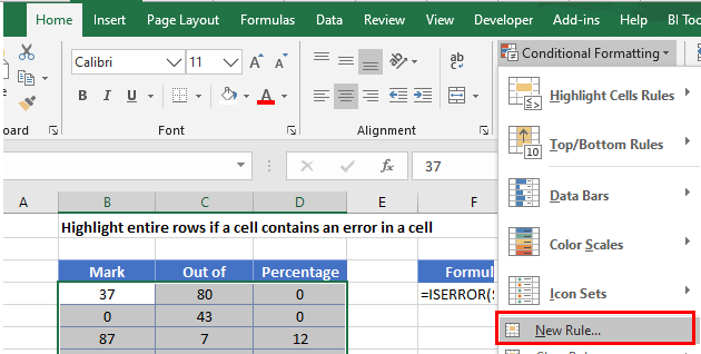
2. In the Ribbon, select Home > Conditional Formatting > New Rule.

 

 

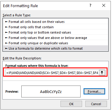
3. Select Use a formula to determine which cells to format, and enter the following formula (with the AND Function):

=IF(AND(AND(AND(AND($C4>$H$6,$D4>$H$6,$E4>$H$6,$F4>$H$6)))),TRUE,FALSE)

 

 

4. You need to use a mixed reference in this formula ($C4, $D4, $E4, $F4) in order to lock the column but make the row relative – this will enable the formatting to format the entire row instead of just a single cell that meets the criteria.
5. When the rule is evaluated, each column is evaluated by a nested IF statement – and if all the IF statements are true, then a TRUE is returned, and the entire row is highlighted. As you are applying the formula to a range of columns and rows, the row changes relatively, but the column will always remain the same.
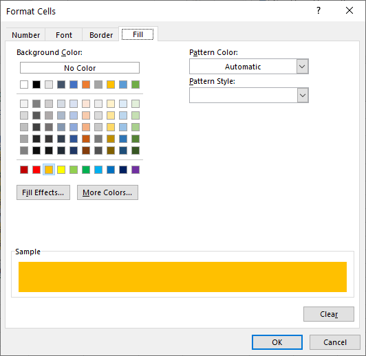
6. Click on the Format button and select your desired formatting.

 

 

7. Click OK, and then OK once again to return to the Conditional Formatting Rules Manager.

 

 

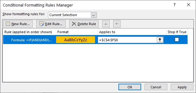
8. Click Apply to apply the formatting to your selected range and then click Close.

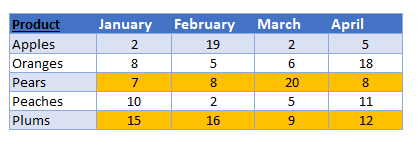
Every row in the range selected that has each cell with a value greater than 5 will have its background color changed to yellow.

 

 

ISERROR Function

To highlight a row if there is a cell with an error in it in the row with conditional formatting, you can use the ISERROR Function within a Conditional Formatting rule.

 

 

1. Select the range you want to apply formatting to.
2. In the Ribbon, select Home > Conditional Formatting > New Rule.

 

 

3. Select Use a formula to determine which cells to format, and enter the following formula:

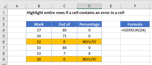
=ISERROR($D4)

 

 

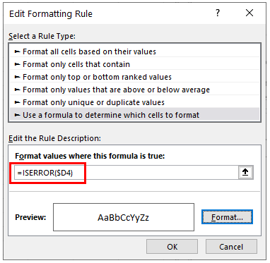
4. You need to use a mixed reference to make sure that the column is locked and that the row is relative – this will enable the formatting to format the entire row instead of just a single cell that meets the criteria.
5. When the rule is evaluated for all the cells in the range, the row will change but the column will remain the same. This causes the rule to ignore the values in any of the other columns and just concentrate on the values in Column D. As long as the rows match, and Column D of that row returns an error, then the formula result is TRUE and the formatting is applied for the whole row.
6. Click on the Format button and select your desired formatting.

 

 

7. Click OK, and then OK once again to return to the Conditional Formatting Rules Manager.

 

 

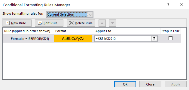
8. Click Apply to apply the formatting to your selected range and then click Close.

 

 

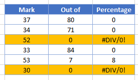
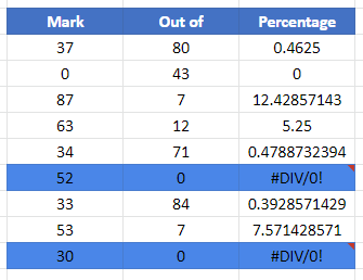
Every row in the range selected that has a cell with an error in it has its background color changed to yellow.

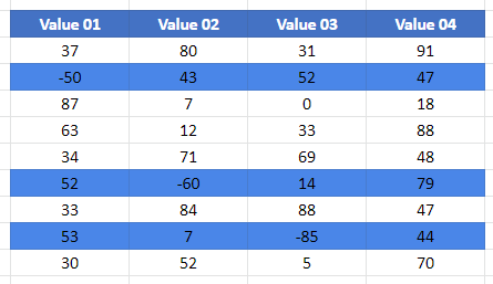
Evaluate for Negative Numbers

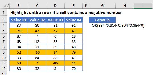
To highlight a row if there is a cell with a negative number in it in the row with conditional formatting, you can use the OR Function within a Conditional Formatting rule.

 

 

1. Select the range you want to apply formatting to.
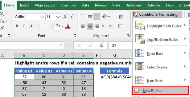
2. In the Ribbon, select Home > Conditional Formatting > New Rule.

 

 

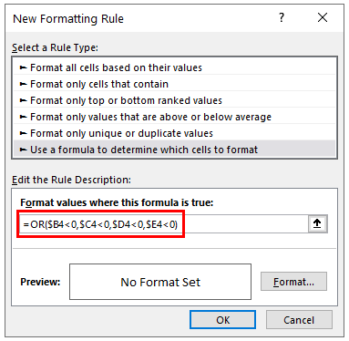
3. Select Use a formula to determine which cells to format, and enter the formula:

=OR($B4<0,$C4<0,$D4<0,$E4<0)

 

 

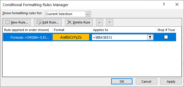
4. You need to use a mixed reference to make sure that the column is locked and that the row is relative – this will enable the formatting to format the entire row instead of just a single cell that meets the criteria.
5. When the rule is evaluated, each column is evaluated by the OR statement – and if all the OR statements are true, then a TRUE is returned. If a TRUE is returned, then the entire formula will return true and the entire row is highlighted. As you are applying the formula to a range of columns and rows, as the row changes, the row in the will change relatively, but the column will always remain the same.
6. Click on the Format button and select your desired formatting.

 

 

7. Click OK, and then OK once again to return to the Conditional Formatting Rules Manager.

 

 

8. Click Apply to apply the formatting to your selected range and then click Close.

 

 

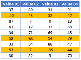
Every row in the range selected that has a cell with a negative number will have its background color changed to yellow.

Conditional Format If in Google Sheets

The process to highlight rows based on the value contained in that cell in Google Sheets is similar to the process in Excel.

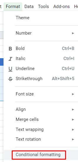
1. Highlight the cells you wish to format, and then click on Format > Conditional Formatting.

 

 

2. The Apply to Range section will already be filled in.

 

 

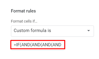
3. From the Format Rules section, select Custom Formula.
4. Type in the following formula.

=IF(AND(AND(AND(AND($C4>$H$6,$D4>$H$6,$E4>$H$6,$F4>$H$6)))),TRUE,FALSE)

 

 

5. Select the fill style for the cells that meet the criteria.

 

 

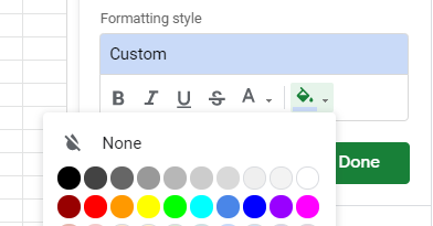
6. Click Done to apply the rule.

See also: IF Formula – Set Cell Color w/ Conditional Formatting.

If There Is an Error

The process to highlight rows where an error is contained in a cell in the row in Google Sheets is similar to the process in Excel.

1. Highlight the cells you wish to format, and then click on Format, Conditional Formatting.

 

 

2. The Apply to Range section will already be filled in.

 

 

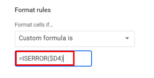
3. From the Format Rules section, select Custom Formula.
4. Type in the following formula:

=ISERROR($D4)

 

 

5. Select the fill style for the cells that meet the criteria.

 

 

6. Click Done to apply the rule.

 

 

Evaluate for Negative Numbers

The process to highlight rows if there is a cell with a negative number in it in the row with conditional formatting sheets is similar to the process in Excel.

1. Highlight the cells you wish to format, and then click on Format > Conditional Formatting.
2. The Apply to Range section will already be filled in.
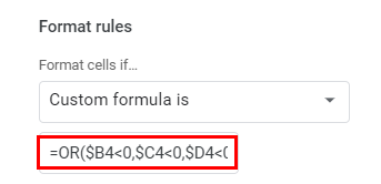
3. From the Format Rules section, select Custom Formula.
4. Type the following formula.

=OR($B4<0,$C4<0,$D4<0,$E4<0)

 

 

5. Select the fill style for the cells that meet the criteria.
6. Click Done to apply the rule.