다음보다 크거나 작은 조건부 서식 – Excel 및 Google 스프레드시트
Last updated on 7월 27, 2023
이 튜토리얼에서는 Excel 및 Google 스프레드시트에서 조건부 서식을 사용하여 셀이 다른 셀보다 크거나 작은지에 따라 셀을 강조 표시하는 방법을 보여 줍니다.
셀 하이라이트 규칙 사용
값이 지정된 숫자보다 큰 셀을 강조 표시하려면 조건부 서식 메뉴에서 기본으로 제공되는 셀 강조 표시 규칙 중 하나를 사용할 수 있습니다.
다음보다 큼
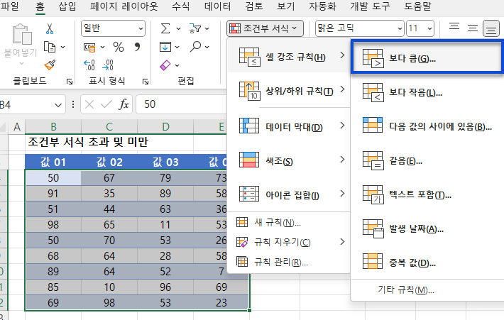
- 서식을 적용할 범위를 선택합니다(예: B4:E12).
- 리본에서 홈 > 조건부 서식 > 셀 강조 규칙 > 보다 큼…을 선택합니다.
- 값을 입력하거나 서식을 동적으로 적용되게 만들기 위해(즉, 값을 변경하면 결과가 변경되도록) 필요한 값이 포함된 셀을 클릭할 수 있습니다.
- 드롭다운 상자에서 필요한 서식 유형을 선택하고 확인을 클릭합니다.
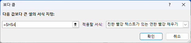
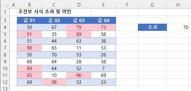
이제 표에서 H4 셀(50)에 있는 값보다 큰 값이 빨간색으로 표시되어 있습니다.
- 다른 결과를 얻으려면 H4의 값을 변경합니다.
다음보다 작음
- 서식을 적용할 범위를 선택합니다.
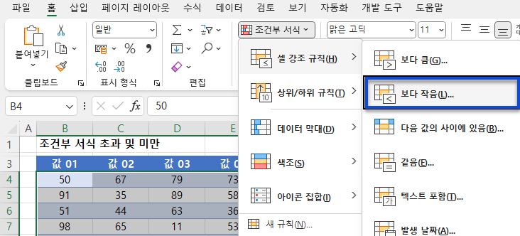
- 리본에서 홈 > 조건부 서식 > 셀 규칙 강조 표시 > 보다 작음...을 선택합니다
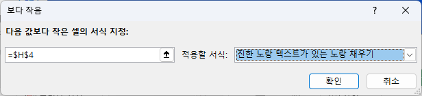
- 이전과 마찬가지로 필요한 값이 포함된 셀을 클릭합니다.
- 확인을 클릭하여 원하는 서식으로 셀의 서식을 지정합니다.
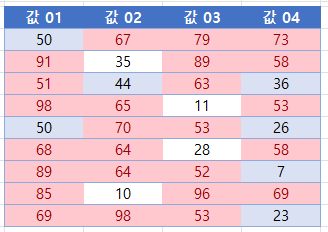
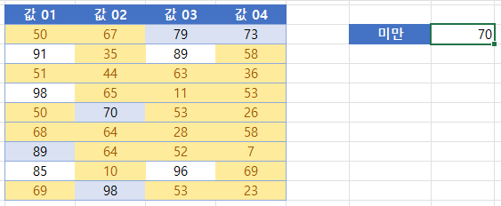
결과 서식은 70보다 작은 숫자를 노란색으로 표시합니다.
사용자 지정 함수로 셀 강조 표시
조건부 서식을 사용하면 사용자 지정 함수를 사용하여 셀을 강조 표시할 수도 있습니다.
다음보다 큼 및 다음보다 작음
새 규칙을 생성하고 수식 사용을 선택하여 서식을 지정할 셀을 결정하면 한개의 특정 셀보다 큰 값을 가지면서 다른 특정 셀보다 작은 값을 가진 셀을 강조 표시할 수 있습니다.
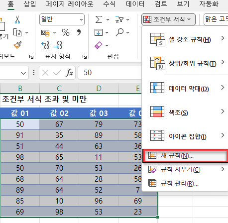
- 서식을 적용할 범위를 선택합니다.
- 리본에서 홈 > 조건부 서식 > 새 규칙을 선택합니다.
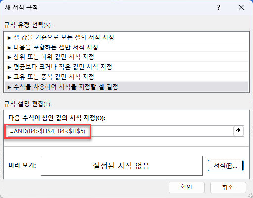
- 수식 사용을 선택하여 서식을 지정할 셀을 결정하고 AND 함수를 사용하기 위해 아래 수식을 입력합니다:
=AND(B4>$H$4, B4<$H$5)- H4 및 H5 셀에 대한 참조를 절대값으로 만들어 고정시켜야 합니다. 행과 열 표시기 주위에 $ 기호를 사용하거나 키보드에서 F4를 눌러 이 작업을 수행합니다.
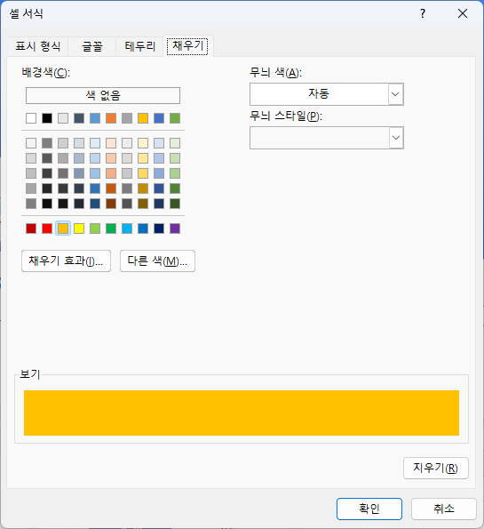
- 마지막으로 서식 버튼을 클릭합니다.
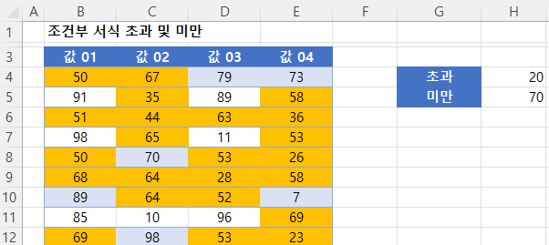
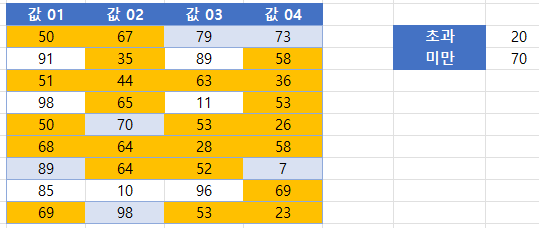
- H4(20)와 H5(70) 사이의 숫자에 대해 원하는 서식을 선택합니다. 확인을 클릭합니다.
결과는 이전 예제와 유사하며 다른 조건에 강조 표시만 됩니다.
다음보다 크거나 다음보다 작음
한 셀보다 값이 크거나 다른 셀보다 값이 작은 셀(즉, 두 셀의 범위를 벗어난 셀)을 강조 표시하려면 다음 단계를 따르세요:
- 서식을 적용할 범위를 선택합니다.
- 리본에서 홈 > 조건부 서식 > 새 규칙을 선택합니다
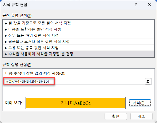
- 수식을 선택하여 서식을 지정할 셀을 결정하고 OR 함수를 사용하기 위해 이 수식을 입력합니다:
=OR(B4>$H$4, B4<$H$5)- 다시 한 번 H4 및 H5 셀에 대한 참조를 절대값으로 만들어 고정시킵니다. 행과 열 표시기 주위에 $ 기호를 사용하거나 키보드에서 F4 키를 누릅니다.
- 서식 버튼을 클릭합니다.
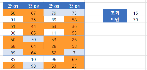
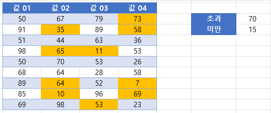
- H4(70)와 H5(15) 사이에 있지 않은 숫자에 대해 원하는 서식을 선택합니다. 확인을 클릭합니다.
Google 스프레드시트에서 사용자 지정 기능으로 셀 강조 표시하기
Google 스프레드시트에서 한 셀보다 큰 값을 가진 셀을 강조 표시하고 다른 셀보다 작은 값을 가진 셀을 강조 표시하는 과정은 Excel의 과정과 유사합니다.
- 서식을 지정하려는 셀을 강조 표시한 다음 서식 > 조건부 서식을 클릭합니다.
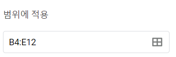
- 범위에 적용 섹션이 이미 채워져 있을 것입니다.
- 서식 규칙 섹션의 드롭다운 목록에서 맞춤 수식을 선택하고 다음 수식을 입력합니다:
=AND(B4>$H$4, B4<$H$5)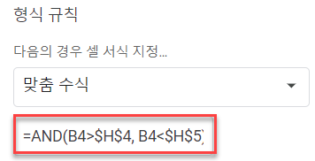
다시 한 번 절대 기호(달러 기호)를 사용하여 H4 및 H5의 값을 고정합니다.
- 기준을 충족하는 셀의 채우기 스타일을 선택합니다.
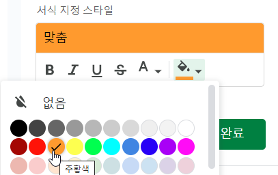
- 완료를 클릭하여 규칙을 적용합니다.