Conditional Formatting – Excel & G Sheets – **Tips for 2023**
Written by
Reviewed by
This tutorial provides an overview of Conditional Formatting in Excel and Google Sheets. Or, scroll to the bottom of the page for 70 tutorials on using Conditional Formatting.
Conditional formatting is a very powerful feature that allows you to automatically apply specific formatting to cells that meet certain criteria and emphasize key attributes of a dataset. Here are some of the most valuable conditional formatting tips.
In this tutorial…
Highlight Cells Rules
Highlight Top Items
Highlight Row Based on Value
Add Data Bars
Add Color Scales
Icon Sets
Manage Conditional Formatting Rules
Hierarchy of Conditional Formatting Rules
Clear Conditional Formatting Rules
Conditional Formatting Rules in Google Sheets
Highlight Cells Rules
The Highlight Cells Rules test each cell they’re applied to against a given condition and formats cells that meet your condition(s). Possibilities for setting these rules is to format cells greater than, less than, or equal to a certain value; between two set values; containing a text string; relating to a certain date; or containing a duplicated value. Below are two examples of Highlight Cells Rules.
Highlight Cells Less Than Certain Value
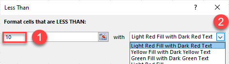
Say you have a data set with products and accompanying information about them. One piece of information is how many pieces of a particular product you have sold, and you want to highlight only the cells with values less than 10.
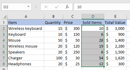
- First, select the range to apply the formatting (e.g., D2:D8).
- Then, in the Ribbon, go to Home > Conditional Formatting > Highlight Cells Rules > Less Than…
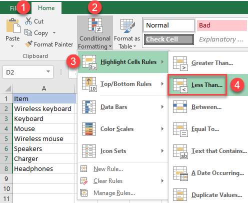
- The Less Than pop-up appears. In the field to the left, enter the desired value (e.g., 10). In the field to the right, select which type of formatting to apply (Light Red Fill with Dark Red Text).
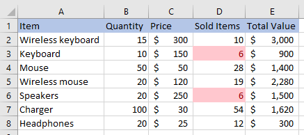
The resulting formatting shows numbers less than 10 in red.
Highlight Cells That Contain Text
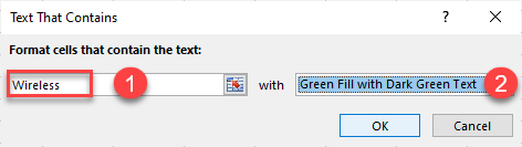
You can use one of the conditional formatting rules to pinpoint where a certain string of text is. Say you have an inventory list and want to highlight all cells that contain the word Wireless.
- Select the data range (e.g., D2:D8).
- In the Ribbon go to Home > Conditional Formatting > Highlight Cells Rules > Text that Contains…
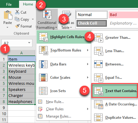
- In the field on the left, enter the text (Wireless), and on the right, select the desired formatting type (Green Fill with Dark Green Text).
Now, all cells with the word Wireless are highlighted in green.
Highlight Top Items
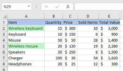
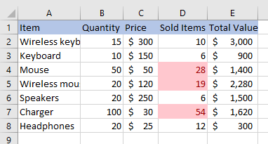
Top/Bottom Rules are a great way to quickly locate the top (or bottom) values from the data. Imagine you have a column with number of products sold and want to highlight the three best-selling products.
- Select the data range (e.g., D2:D8).
- In the Ribbon go to Home > Conditional Formatting > Top/Bottom Rules > Top 10 Items…
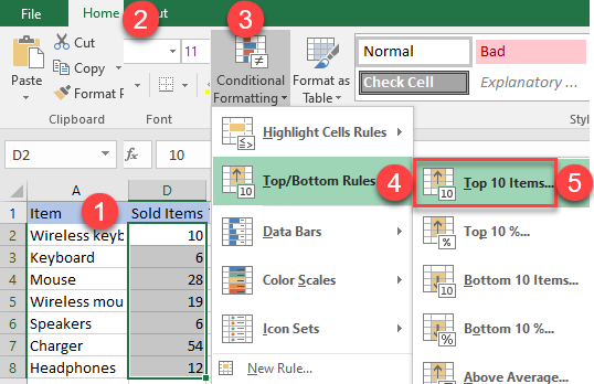
- In the field to the left, click on the arrow to change the number of items from the top. In the field to the right, choose the desired formatting type.
If you want to use your own formatting style, select Custom Format and create one.
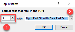
The resulting formatting shows the top three values in red.
Highlight Entire Row Based on Cell Value
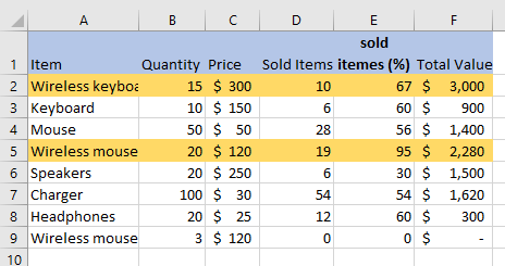
Sometimes, it is much easier to recognize important data when you highlight the whole row instead of a single cell. Say you have a percentage of products sold and want to highlight the entire row when the percentage is greater than 60.
- First, select the data range (e.g., A1:F9).
- In the Ribbon, go to Home > Conditional Formatting > New Rule…
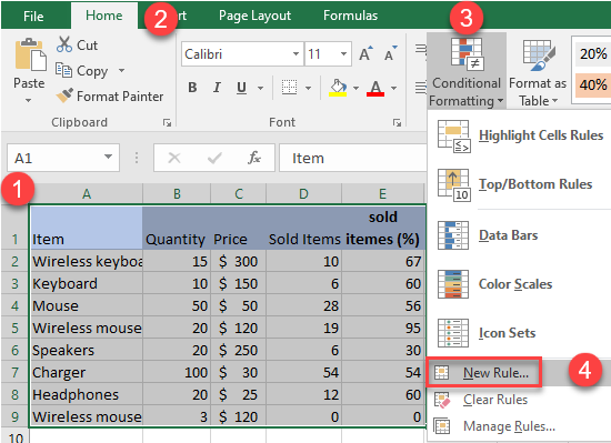
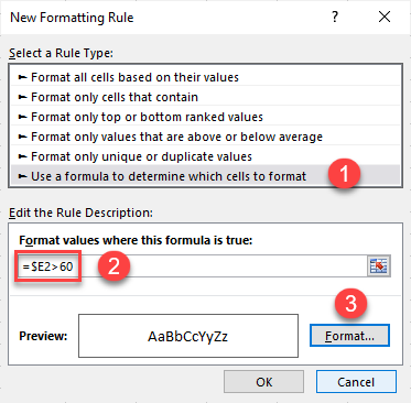
- The New Formatting Rule window opens. As the rule type, choose Use a formula to determine which cells to format. Below that, enter the formula:
=$E2 > 60Then press Format.
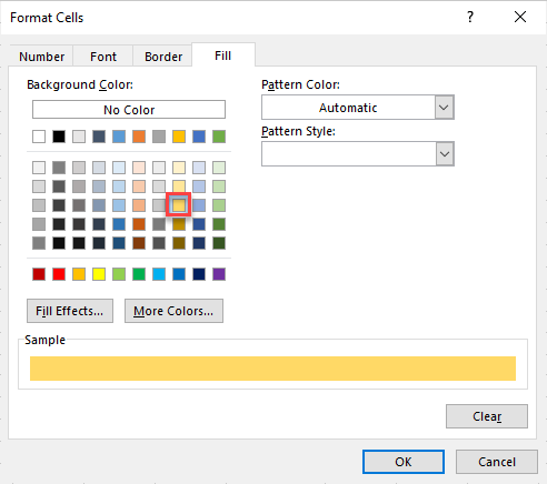
- In the Format Cells window, choose a fill color and press OK.
For each cell in Column F that has a value greater than 60, the entire corresponding row is highlighted in yellow.
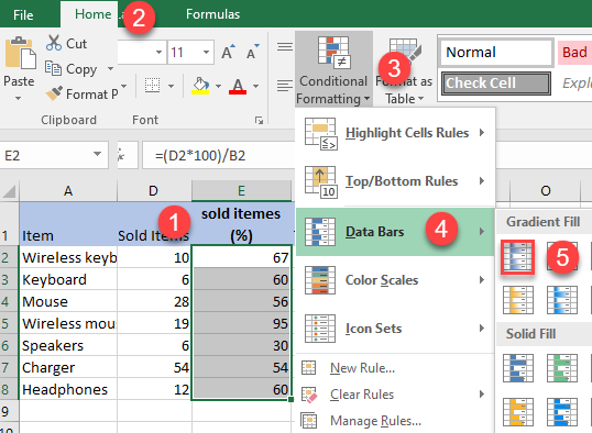
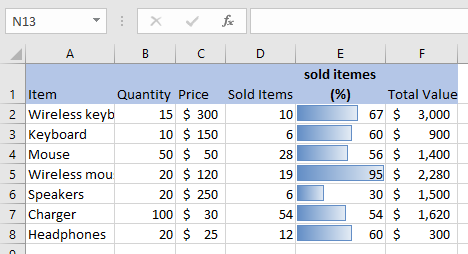
Add Data Bars
Using data bars is a simple way to visually represent the top and bottom values of your data and it is a very effective tool when working on larger datasets.
A data bar’s length in a cell is determined by the values of the other selected cells; the bar is long if the value is high in comparison to the rest of the cells, and vice versa.
- Select the data range (e.g., E2:E8).
- In the Ribbon, go to Home > Conditional Formatting > Data Bars. Choose a formatting option (choose between gradient and solid fill and choose a color).
As a result, bars are added to each cell. The eye is immediately drawn to the highest value, and the amounts can be compared visually.
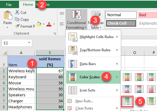
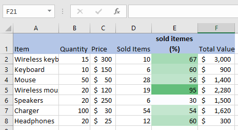
Add Color Scales
Using color scales is very similar to using data bars. The only difference is in the visual representation.
The cell with the highest value is assigned a color, the cell with the lowest value is assigned with another one, and all cells in between are assigned a mix of these two colors. You can also choose formatting with three colors; the middle value would be assigned to the third color.
- Select the data range (e.g., E2:E8).
- In the Ribbon, go to Home > Conditional Formatting > Data Bars. Choose a formatting option. You can choose a color scheme and the order of colors/shades from the default options or create your own.
The resulting formatting shows selected cells with assigned colors.
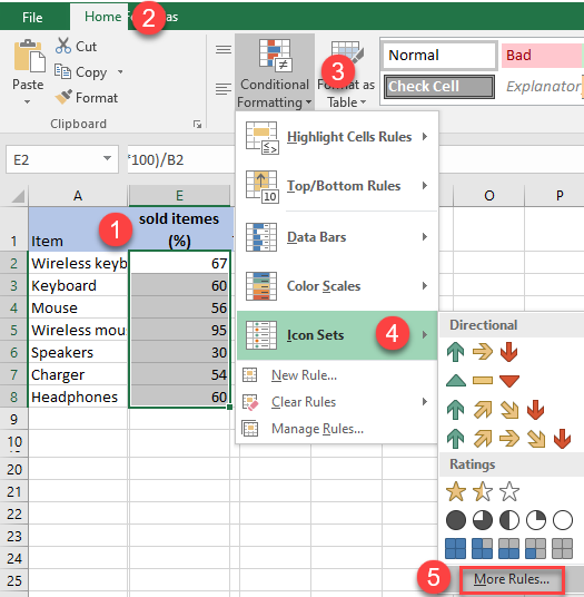
Icon Sets
Conditional formatting icon sets are a great feature to help you visually represent data with shapes, arrows, checkmarks, or other objects.
- Select the data (e.g., E2:E8).
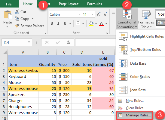
- In the Ribbon, go to Home > Conditional Formatting > Icon Sets.
Choose one of presets (the icons will appear in the inside selected cells straightaway) or click on More Rules… to customize the icon sets.
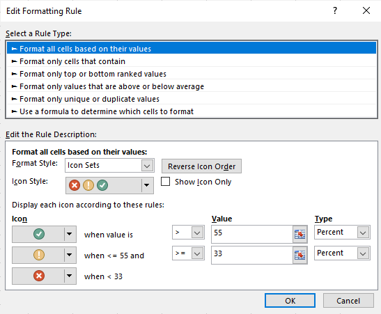
Checkmarks
You can also depict the data using checkmarks.
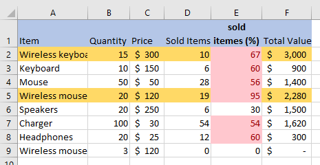
Assign cells with a value greater than 67 green checkmark icons, cells with a value between 33 and 67 yellow exclamation icons, and cells with a value less than 33 red X icons.
- Select the data (e.g., E2:E8).
- In the Ribbon, go to Home > Conditional Formatting > Icon Sets > More Rules…
- Choose Icon Sets as format style.
- Then choose the desired icon style (checkmark, exclamation point, X) from the drop-down menu.
- To set a rule, enter values (67 and 33) in the Value boxes.
- Choose the correct type of values (Percent because the selected data is expressed as percentages).
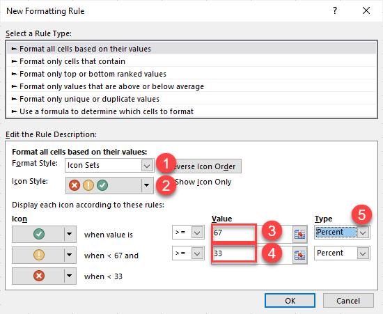
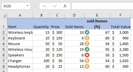
As a result, all cells with a value greater or equal to 67 will have a green checkmark icon in them, all cells with a value less than 67 and greater or equal to 33 will have a yellow exclamation icon, and cells with a value less than 33 will have red X icon.
Manage Conditional Formatting Rules
If you want to make a change in a conditional formatting rule, you can easily do so using the Conditional Formatting Rules Manager.
- Select the data range (e.g., A1:F9).
- In the Ribbon go to Home > Conditional Formatting > Manage Rules…
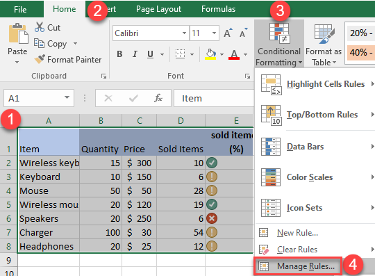
- The Conditional Formatting Manager window opens. Double-click on the rule you want to change.
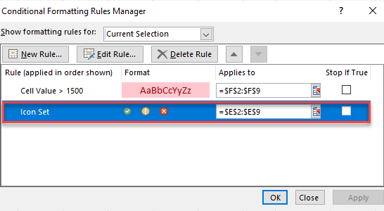
- This brings up the Edit Formatting Rule window. Once you make all necessary changes, press OK.
You can also use the Conditional Formatting Rules Manager to change the hierarchy of the rules, delete them, or make new ones.
Hierarchy of Conditional Formatting Rules
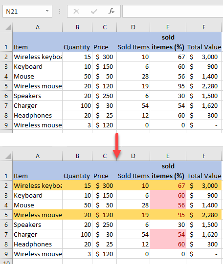
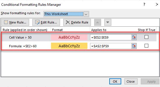
Using more than one conditional formatting rule at the same time can cause problems because of overlapping. Say you have two rules:
- First rule: Highlight all cells with cell values greater than 50.
- Second rule: Highlight the entire row if the value in Column E is greater than 60.
In this case, the second rule row formatting is only applied to cells without the first rule cell formatting, as shown in the picture below.
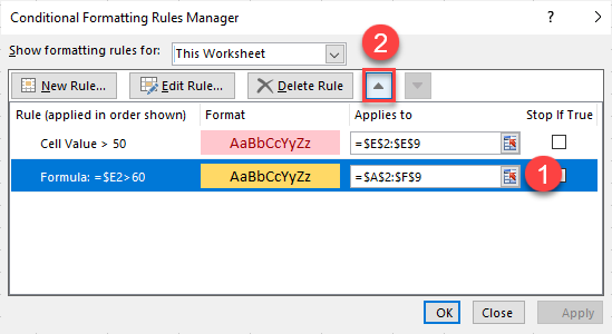
If you want to give preference to the second rule, you’ll have to change the hierarchy of the rules.
- In the Ribbon go to Home > Conditional Formatting > Manage Rules…
- This opens the Conditional Formatting Rules Manager window, which shows the current hierarchy of your rules.
- To raise the second rule to the top, select it and press the up arrow next to “Delete Rule.” Press OK to finish.
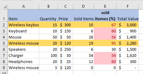
The hierarchy will change, and as a result, rows are highlighted without interruption at the overlap points. Row highlighting supersedes cell highlighting, but since the (red) cell formatting also changes the font color, cells where both conditions apply are highlighted in orange with red font.
Clear Conditional Formatting Rules
Sometimes, you’ll end up with a worksheet with too many conditional formatting rules. That could cause the formatting to be faulty, not matching its intent, or slow down Excel. To fix that, you can delete some (or all) of the conditional formatting rules.
Delete All Rules
To delete all conditional formatting rules, in the Ribbon go to Home > Conditional Formatting > Clear Rules > Clear Rules from Entire Sheet.
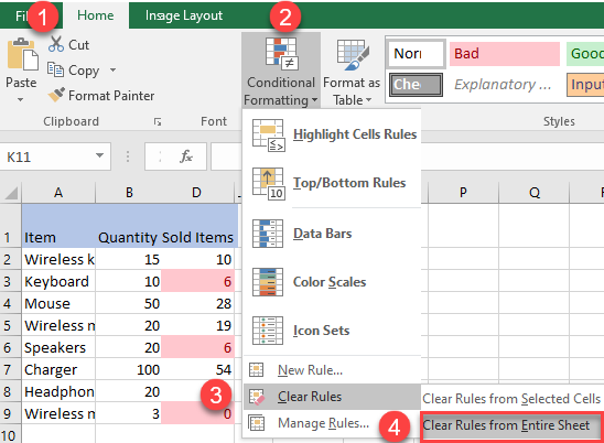
If you select a certain data range and you want to delete rules for that range, choose Clear Rules from Selected Cells, instead of from the entire sheet.
Delete Specific Rules
To specifically select which rules you want to delete, use the Manage Rules option.
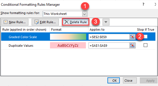
- In the Ribbon go to Home > Conditional Formatting > Manage Rules…
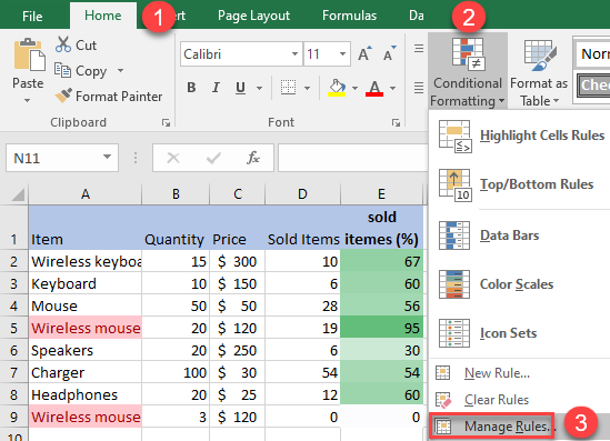
- First select This Worksheet in the Show formatting rules for section.
- Then select the rule you want to remove and press the Delete rule icon. Then, click OK.
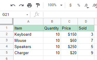
Conditional Formatting Rules in Google Sheets
You can also use conditional formatting rules in Google Sheets to format cells that meet certain criteria, but there are fewer options than there are in Excel.
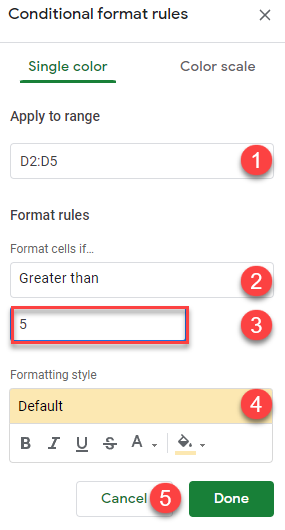
In the Menu, go to Format > Conditional formatting.
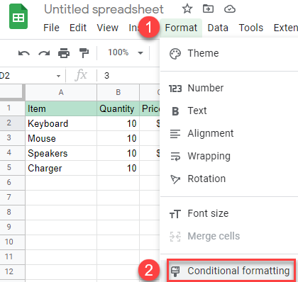
The Conditional format rules pane opens on the right side of the sheet. There are two options for conditional formatting in Google Sheets:
- Single color: Use this option to highlight all cells in a single color.
- Color scale: Use this option to visually present the difference between the values in the cells.
- Select the data range in the sheet or enter it manually in the box.
- Choose the desired format rule from the list.
- In the next box down, enter the text or formula.
- Now, choose the desired formatting style.
- When finished, press Done.
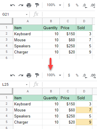
Clear Conditional Formatting Rules in Google Sheets
To clear conditional formatting rules in Google Sheets:
- Select the data range (e.g., A1:A5).
- In the Menu go to Format > Clear formatting.
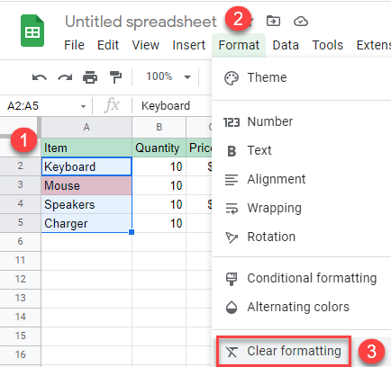
As a result, all conditional formatting rules for the selected range are deleted.