How to Use Comparison Icon Sets in Excel & Google Sheets

This tutorial will demonstrate how to use conditional formatting comparison icon sets to compare data visually in Excel and Google Sheets.

 

 

Conditional Formatting Icon Sets

Comparison icon sets are useful for seeing trends in prices, stock markets, shares etc. Icon sets are a type of conditional formatting that allows you to compare cell values with other cells and show data trends.

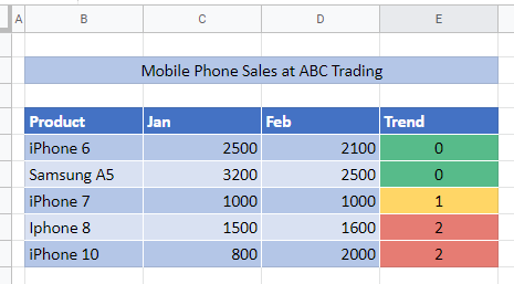
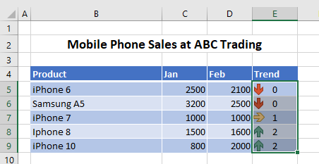
Consider the following worksheet.

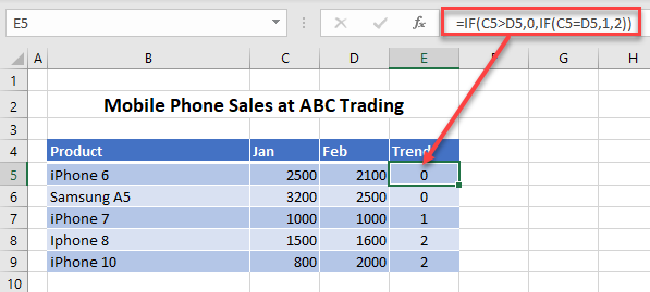
The data for the sales of mobile phones for January and February is in the worksheet. The trend is to see if the February sales are greater than the January sales. Column E is 0 if the sales have decreased, 1 if they have stayed the same, and 2 if they have increased.

 

 

Directional Icon Set

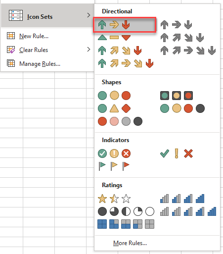
1. To apply comparison icon set formatting, start by highlighting the cells to be compared (E5:E8). In the Ribbon, select Home > Styles > Conditional Formatting > Icon Sets.

 

 

2. There are a variety of different icon sets to select from. For this example, select Directional to show the trend.

 

 

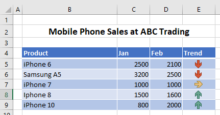
The conditional formatting rule is applied to the selected cells.

 

 

3. To remove the 0 and 1 from the cells, edit the applied conditional formatting rule.
   In the Ribbon, select Home > Styles > Conditional Formatting > Manage Rules.

 

 

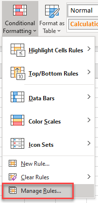
4. Select the Icon Set rule, and then click Edit Rule.

 

 

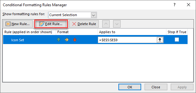
5. Check the box next to “Show Icon Only“. You can also customize the icon set that is used for the rule – to see how to do this, click here.
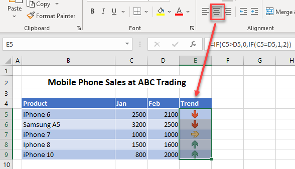
6. Click OK twice to return to Excel.

 

 

7. Then center the icons in the cells.

 

 

Shapes Icon Set

1. You can also use the Shapes Icon sets to apply “traffic light” icons to the data.

 

 

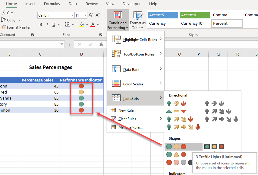
The color of the indicators is based on the values that are stored in the icon set rule.

2. To amend these values, in the Ribbon, select Home > Styles > Conditional Formatting > Manage Rules.

 

 

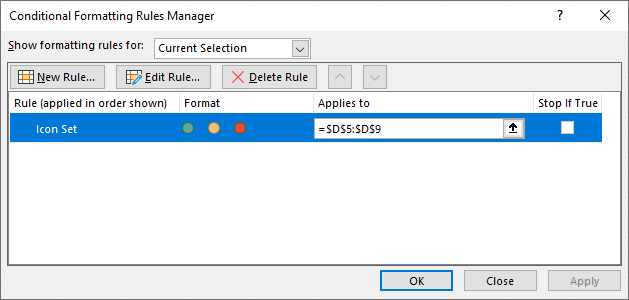
3. Select the required rule, then select Edit rule.

 

 

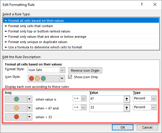
4. Edit the values if required, and then click OK twice to return to Excel.

See also…

• Using Conditional Formatting with Excel VBA
• How to Use Custom Icon Sets in Excel & Google Sheets
• How to Insert Harvey Balls in Excel & Google Sheets

Comparison Icon Sets in Google Sheets

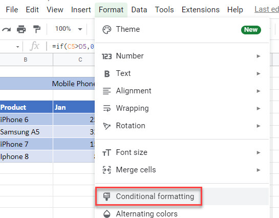
Google Sheets does not have icon sets in conditional formatting. You can, however, apply color codes to your data.

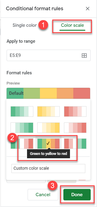
1. Select the data you wish to color code. In the Menu, select Format > Conditional Formatting.

 

 

2. Select Color scale and then select the scale you want to use. Finally click Done.

 

The conditional formatting rule is applied to the data.