How to Use Custom Icon Sets in Excel & Google Sheets
Written by
Reviewed by
This tutorial will demonstrate how to use custom icon sets in Excel and Google Sheets.
Customize Conditional Formatting Icon Sets
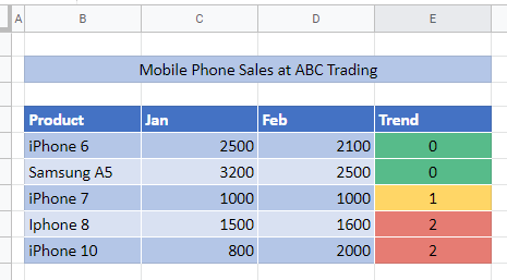
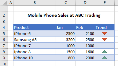
Comparison icon sets in Excel are useful for seeing trends in prices, stock markets, shares etc. Icon sets are a type of conditional formatting that allows you to compare cell values and show their differences. Conditional Formatting in Excel carries standard icon sets you can customize to fit your data and needs.
Once you’ve formatted cells with a standard icon set, you can edit the conditional formatting rule to amend the way the icon sets display.
- Select the cells where the Conditional Formatting rule is applied.
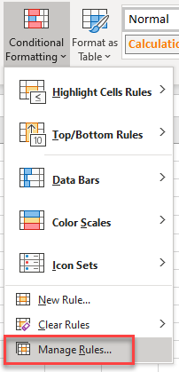
- In the Ribbon, select Home > Styles > Conditional Formatting > Manage Rules.
- Select the Icon Set rule, and then click Edit Rule.
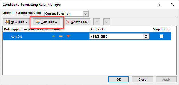
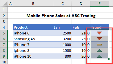
- Then either edit or remove the cell icon for the middle value.
![]()
- Click OK, then OK again to return to Excel.
Note: You can also customize and use icon sets with VBA.
Custom Icon Sets in Google Sheets
Google Sheets does not have icon sets in conditional formatting. You can, however, apply color codes to the data. See How to Use Comparison Icon Sets for the process.