Conditional Formatting Based on Cell Value / Text – Excel & Google Sheets

This tutorial demonstrates how to apply conditional formatting based on a cell value or text in Excel and Google Sheets.

 

 

Excel has a number of built-in Conditional Formatting rules that can be used to format cells based on the value of each individual cell.

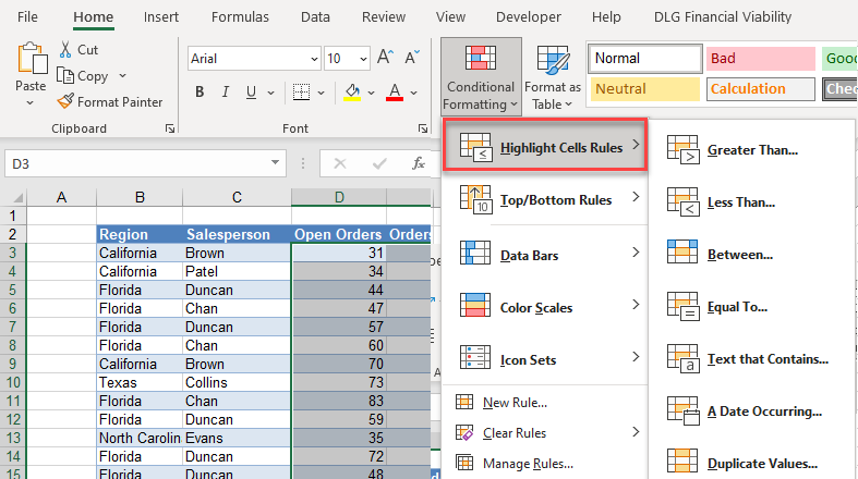
Highlight Cells Rules

Perhaps the most straightforward set of built-in rules simply highlights cells containing values or text that meet criteria you define.

1. Select the cells where you want to highlight certain values.

 

 

2. Then, in the Ribbon, select Home > Conditional Formatting > Highlight Cells Rules.
   The Highlight Cells Rules category allows you to select from greater than, less than, or equal to a certain value; between two set values; containing a text string; relating to a certain date; or containing a duplicated value.

 

 

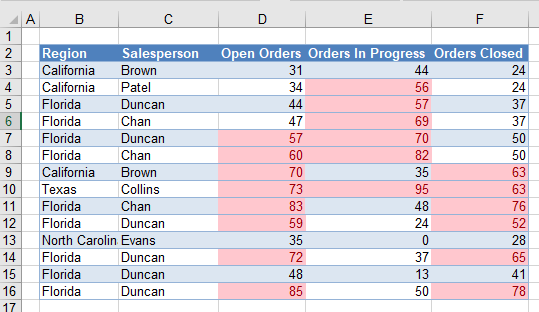
3. For this example, select Greater Than… and then type in the target number, where you want cells greater than that target highlighted, and select a format.

 

 

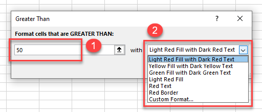
Note: Instead of typing in the actual value in the Format cells that are GREATER THAN box, you can click on a cell in your worksheet where you have a value stored. This would mean that if the value in that cell on your worksheet changed, the conditional formatting would change.

4. Click OK.

 

 

Highlight Cells With Text

You can also test whether a cell contains a certain word or string of text using Highlight Cells Rules.

1. Once again, select the cells where you want to highlight based on text.
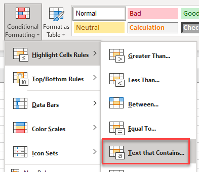
2. Then, in the Ribbon, select Home > Conditional Formatting > Highlight Cells Rules > Text that Contains…

 

 

3. Type in your target text and select a format.

 

 

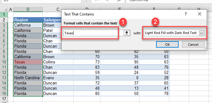
4. Click OK.

Note: you can also type in part of a word or part of the text that is in the cell, you do not have to match the text entirely so typing as, for example, finds the cell with Texas in it.

Custom Rule

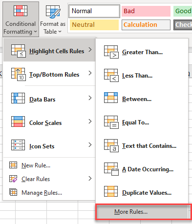
1. In addition to these built-in Highlight Cells Rules, you can also create a custom rule by clicking on the More Rules… option at the bottom of the Highlight Cells Rules menu.

 

 

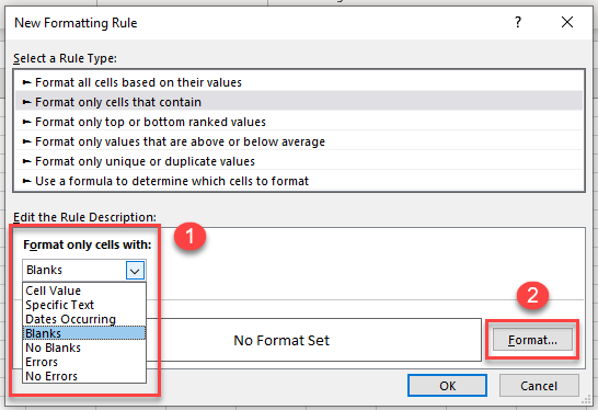
2. Format only cells that contain is already highlighted. For this example, in the Format only cells with drop-down box, select Blanks.
3. Then click Format…

 

 

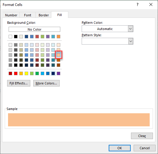
4. In the Format Cells window, choose a fill color, and press OK.

 

 

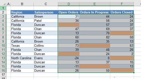
5. Click OK once again to apply the conditional formatting to your cells.

 

 

Top/Bottom Rules

Top and bottom rules allow you to format cells according to the top or bottom values in a range. These rules only work on cells that contain values (not text!).

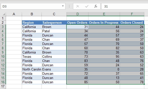
1. Select the range where you want to highlight the highest or lowest values.
2. Then, in the Ribbon, select Home > Conditional Formatting > Top/Bottom Rules.

 

 

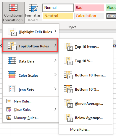
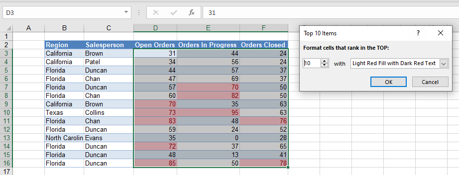
The Top/Bottom Rules category allows you to select from Top 10 Items, Top 10%, Bottom 10 Items, Bottom 10%, Above Average, or Below Average.

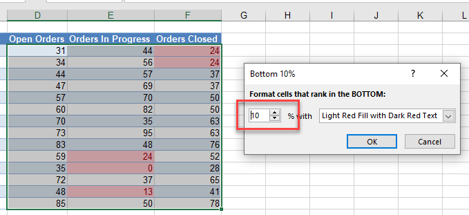
3. For this example, select Bottom 10%…
4. Adjust the target percentage up or down as needed, and then select a format. Click OK to apply the format to selected cells.

 

 

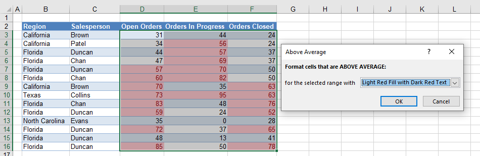
Note that you could also select Above Average or Below Average. These rules automatically calculate the mean of your data range and format cells either greater than or less than that value.

 

 

5. To customize your rule even further, go back to the Top/Bottom Rules menu (from Step 2), and click More Rules… at the bottom.

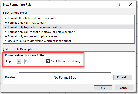
6. The rule type is selected for you (Format only top or bottom ranked values).
   You can then edit the rule description by selecting either Top or Bottom in the drop-down list, and then typing in the comparison value (for example, 25, as shown below).
   Check the % of the selected range if you want the top percentage of the values formatted rather than the actual top 25 values formatted.

 

 

7. Set the format (see Steps 4 and 5 in the “Custom Rule” section), and then click OK to return to Excel.

Data Bars

Data-bars rules add bars to each cell. The higher the value in the cell, the longer the bar is. These rules only work on cells that contain values (not text!).

1. Select the cells where you want to show data bars.
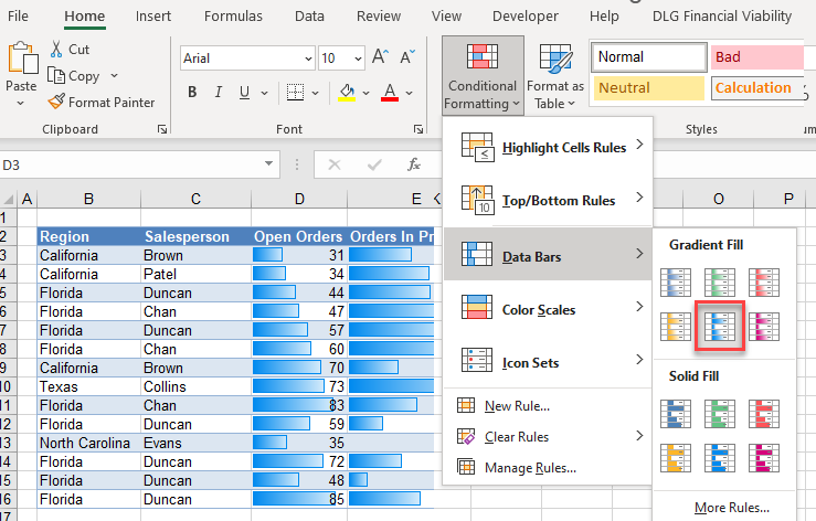
2. Then, in the Ribbon, select Home > Conditional Formatting > Data Bars.

 

 

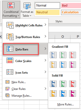
Data-bars rules allow you to select either a Gradient Fill or a Solid Fill bar in a variety of colors.

3. To insert data bars into your cells, click on your preferred option.

 

 

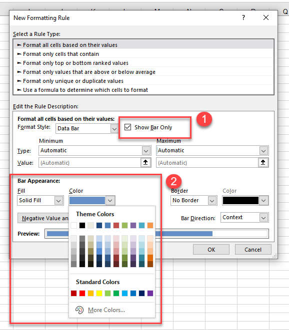
4. To customize your rule even further, click More Rules… at the bottom of the Data Bars menu.
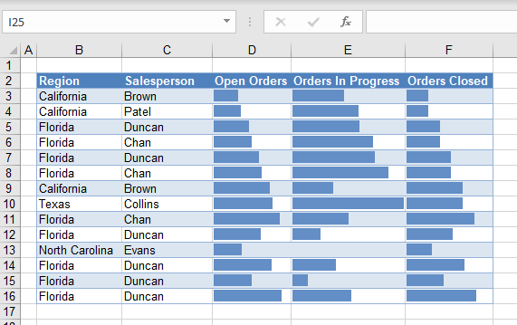
5. The rule type is selected for you (Format all cells based on their values). For this example, check Show Bar Only, and then select the bar appearance (gradient or solid color). You can also choose to add border and choose the direction of the bars.

 

 

6. Click OK to apply the formatting to selected cells.

 

 

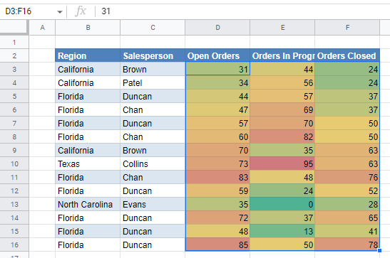
Color Scales

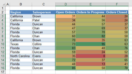
Color-scales rules format cells according to their values relative to a selected range.

1. Select the cells where you want to apply color scales.
2. Then, in the Ribbon, select Home > Conditional Formatting > Color Scales.

 

 

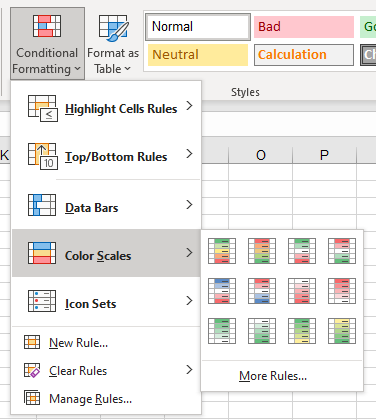
3. To add a color scale to your cells, click on your preferred option.

 

 

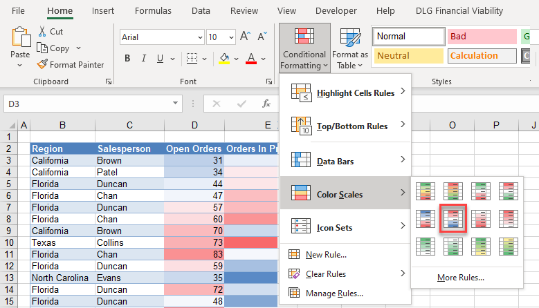
4. To customize your rule even further, click More Rules… at the bottom of the Color Scales menu.
5. The rule type is selected for you (Format all cells based on their values). Select a format style (either 2- or 3-color scale) and then set the values and colors you want.

 

 

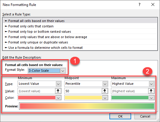
6. Click OK to apply the formatting to your selected cells.

 

 

Icon Sets

There is one more built-in set of rules called Icon Sets. Click the link to learn about adding icon sets to your data.

Format Based on Value or Text in Google Sheets

There are only two types of conditional formatting in Google Sheets: Single color and Color scale. Google Sheets’s Single color rules are similar to Highlight Cells Rules in Excel. Color scales rules are similar in the two applications as well.

Single Color

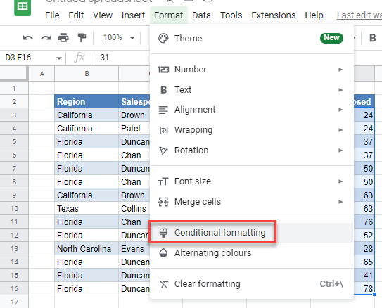
1. Highlight the cells you wish to format, and then in the Menu, select Format > Conditional formatting.

 

 

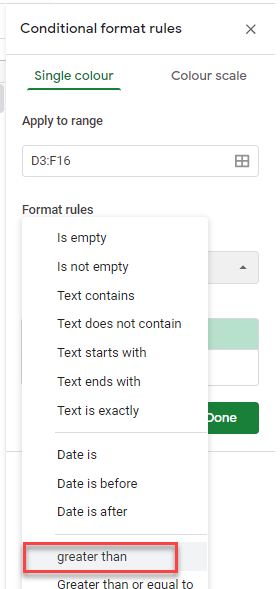
2. In the format rules drop-down box, there is a long list of formats you can apply. For this example, select greater than.

 

 

3. Type in the comparison value, and then click on the format drop down to select a fill color.

 

 

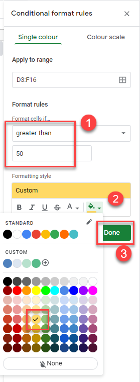
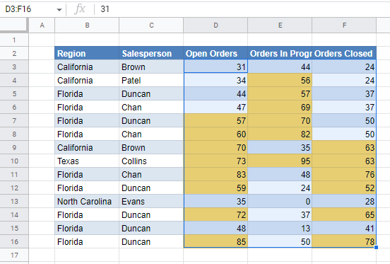
4. Finally, click on Done to apply the formatting to selected cells.

 

 

Color Scale

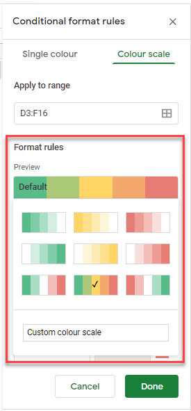
1. To set a Color scale rule, click on Color scale in the Conditional formatting menu. In the format rules box, select an option to preview.

 

 

2. You can then customize the Minpoint, Midpoint, and Maxpoint if you wish, or leave the default values.

 

 

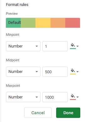
3. Click Done to apply the formatting to your selected cells.