Conditional Formatting If Between Two Numbers – Excel & Google Sheets

This tutorial will demonstrate how to highlight cells that contain a value between two other specified values in Excel and Google Sheets.

 

 

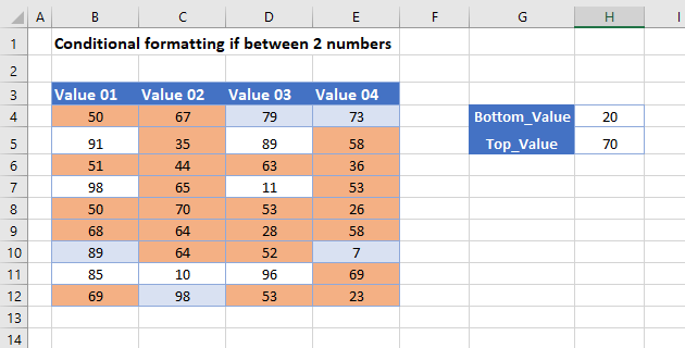
Conditional Formatting if Between Two Numbers

To highlight cells where the value is between a set minimum and maximum (inclusive), you can use one of the built-in Highlight Cell Rules within the Conditional Formatting menu.

1. Select the range you want to apply formatting to.
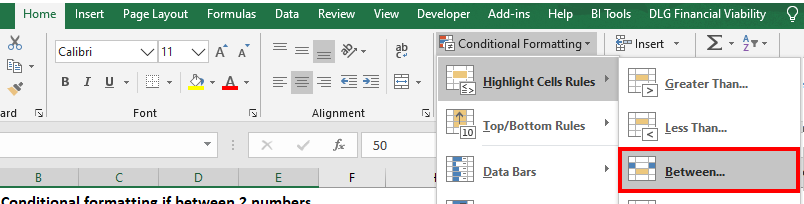
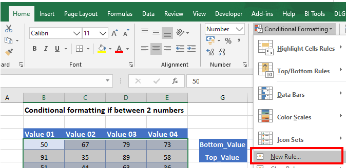
2. In the Ribbon, select Home > Conditional Formatting > Highlight Cells Rules > Between…

 

 

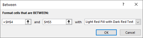
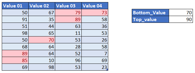
3. You can either type in the bottom and top values, or to make the formatting dynamic (i.e., the result will change if you change the cells), click on the cells that contain the bottom and top values. Click OK.

 

 

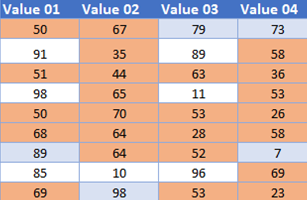
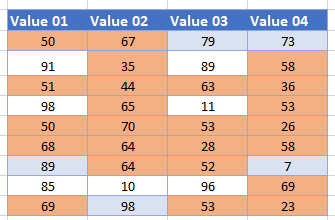
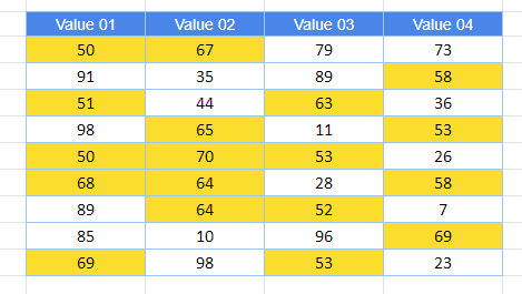
Values between 20 and 70 (inclusive) are highlighted.

 

 

4. When you change the two values in Cells H4 and H5, you obtain a different result.

 

Alternate Method – Custom Formula

You can also highlight cells between two specified numbers by creating a New Rule and selecting Use a formula to determine which cells to format.

1. Select New Rule from the Conditional Formatting menu.

 

 

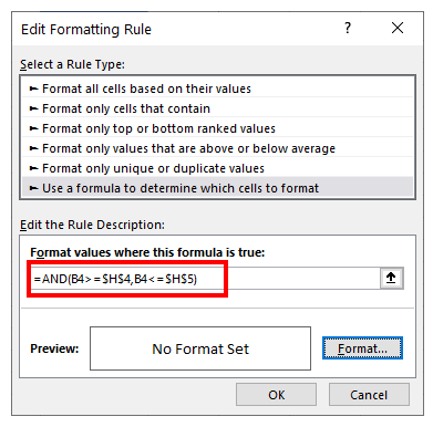
2. Select Use a formula to determine which cells to format, and enter the formula (using the AND Function):

=AND(B4>=$H$4, B4<=$H$5)

3. The reference to cells H3 and H5 need to be locked by making them absolute. You can do this by using the $ sign around the row and column indicators, or by pressing F4 on the keyboard.
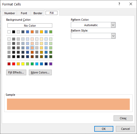
   To learn more about how symbols are used in Excel, see How to Insert Signs and Symbols.
4. Click on the Format button.

 

 

5. Choose a fill color for the highlighted cells.

 

 

6. Click OK, then OK again to return to the Conditional Formatting Rules Manager.

 

 

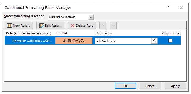
7. Click Apply to apply the format to your worksheet.

 

 

Highlight Cells Between Two Numbers in Google Sheets

Highlighting cells between two numbers in Google Sheets is similar.

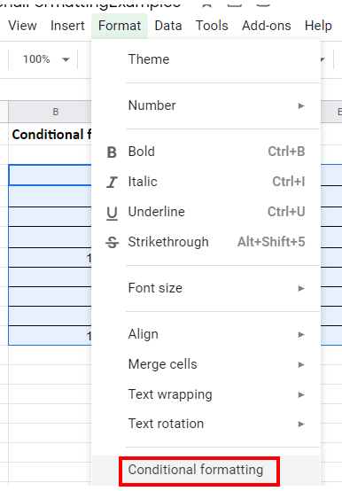
1. Highlight the cells you wish to format, and then click on Format > Conditional Formatting.

 

 

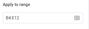
2. The Apply to Range section will already be filled in.

 

 

3. From the Format Rules section, select Is Between from the drop-down list and set the minimum and maximum values.

 

 

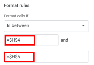
4. Once again, you need to use the absolute signs (dollar signs) to lock in the values in Cells H4 and H5.
5. Select the fill style for the cells that meet the criteria.

 

 

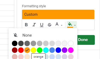
6. Click Done to apply the rule.

 

 

Custom Formula in Google Sheets

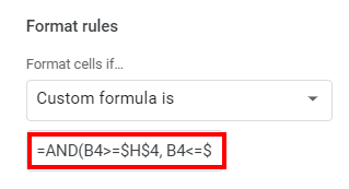
1. To use a custom formula rather than a built-in rule, select Custom formula is under Format Rules, and type the formula.

=AND(B4>=$H$4, B4<=$H$5)

 

 

Remember to use $s or the F4 key to make Cells H4 and H5 absolute.

2. Select your formatting and click Done.