Apply Conditional Formatting to Dates in Excel & Google Sheets

This tutorial demonstrates how to apply conditional formatting to date values in Excel and Google Sheets.

 

 

Apply Conditional Formatting to Dates

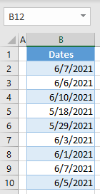
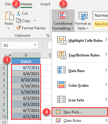
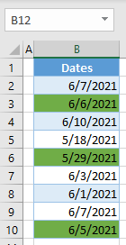
In Excel, you can apply different conditional formatting rules to dates, using built-in options and formulas. Let’s first see how to highlight (in red) dates occurring in the last week. For this example, assume today is 6/7/2021. So the past week is the date range: 5/31/2021–6/6/2021. Below is the list of dates in Column B.

 

 

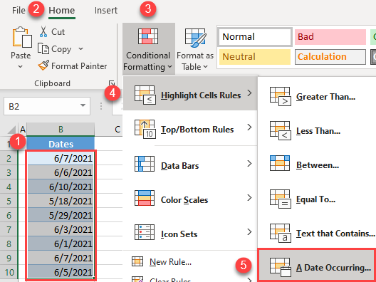
1. Select the range of dates (B2:B10), and in the Ribbon, go to Home > Conditional Formatting > Highlight Cells Rules > A Date Occurring.

 

 

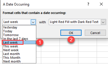
2. In the pop-up window, choose Last week from the drop-down menu and click OK. As you can see, there are other options in the list (Yesterday, Today, Tomorrow, etc.) as well.

 

 

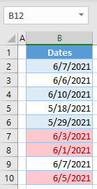
As a result, cells with dates within the last week are highlighted red (B7, B8, and B10).

 

 

Highlight Dates in a Date Range

Now, to highlight dates less than 5 days ago (in this case, 6/3/2021 – 6/6/2021), use the AND Function and TODAY Function .

1. Select the range of dates and in the Ribbon, go to Home > Conditional Formatting > New Rule.

 

 

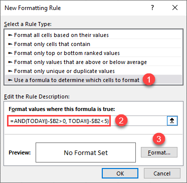
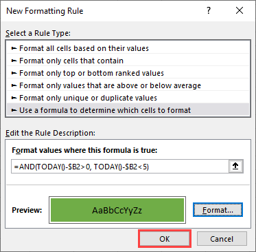
2. In the New Formatting Rule window, (1) select Use a formula to determine which cells to format as the Rule Type and (2) enter the formula:

=AND(TODAY()-$B2>0, TODAY()-$B2<5)

Then (3) click Format.

 

 

This formula goes cell-by-cell, checking whether the difference between today and the date in each cell is greater than 0 and less than 5. If both conditions apply, the result of the formula is TRUE, and the conditional formatting rule is applied. This means that the date in a green cell is in the last 5 days.

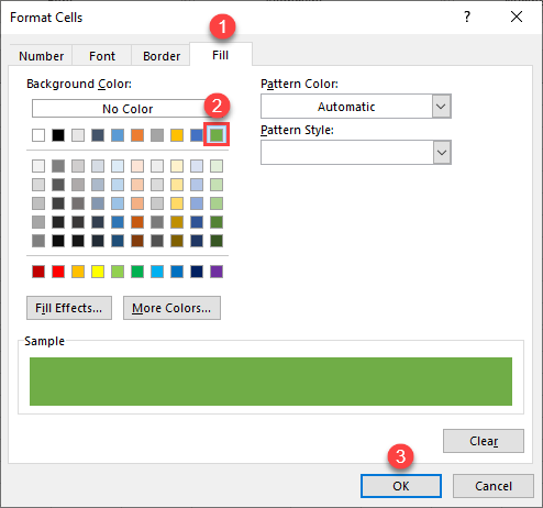
3. In the Format Cells window, go to the Fill tab, select a color (green), and click OK.

 

 

4. This takes you back to the New Formatting Rule window, where you can see a Preview of the formatting and click OK to confirm.

 

 

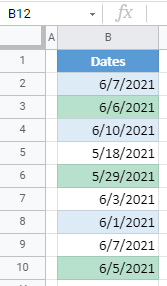
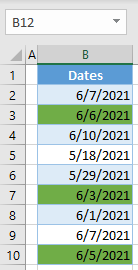
As a result, dates in the last 5 days (here, the current date is 6/7/2021) are highlighted in green (B3, B7, and B10).

 

 

Highlight Weekends

You can also use conditional formatting to highlight dates that fall on Saturdays and Sundays, using the WEEKDAY Function.

1. Select the range with dates (B2:B10), and in the Ribbon, go to Home > Conditional Formatting > New Rule.

 

 

2. In the New Formatting Rule window, (1) select Use a formula to determine which cells to format for a Rule type and (2) enter the formula:

=WEEKDAY($B2,2)>5

Then (3) click Format.

 

 

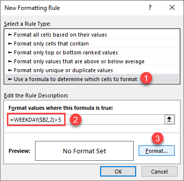
The WEEKDAY Function returns the number of the day in a week. The second parameter value 2, means that the week starts at Monday (1) and ends at Sunday (7). Therefore, for every cell in a range, you are checking if the weekday is greater than 5, which means that the date is on Saturday or Sunday. If that’s true, the conditional formatting rule is applied.

3. In the Format Cells window, (1) go to the Fill tab, (2) select a color (green), and (3) click OK.

 

 

4. This takes you back to in the New Formatting Rule window, where you can see the preview of the formatting and click OK to confirm.

 

 

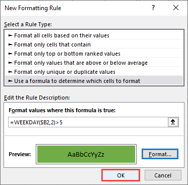
Now, all dates occurring on weekends are highlighted in green (B3, B6, and B10).

 

 

Apply Conditional Formatting to Dates in Google Sheets

You can also use conditional formatting to highlight dates in Google Sheets. To highlight dates in the past week follow these steps:

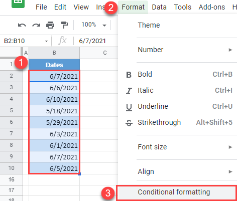
1. Select the range of dates (B2:B10), and in the Menu, go to Format > Conditional formatting.

 

 

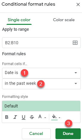
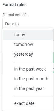
2. On the right side of the window, (1) select Date is for Format rules, (2) choose In the past week, and (3) click Done. This leaves the default color, green, but if you want to change it, you can click on the Fill color icon.

 

 

The result is almost the same as in Excel. Note that Google Sheets, the past week includes today.

 

 

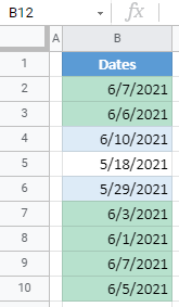
In addition to “past week,” there are other options that can be selected with this formatting rule.

 

 

Highlight Weekends in Google Sheets

As in Excel, you can use formulas in Google Sheets to create more complex rules for conditional formatting.

1. Select the range of dates and in the Menu, go to Format > Conditional formatting.

 

 

2. In the rules window on the right, (1) select Custom formula is for Format rules and (2) enter the formula:

=WEEKDAY($B2,2)>5

Then (3) click Done.

 

 

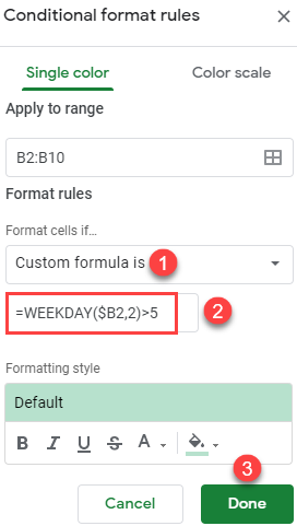
The formula works exactly the same as in Excel, returning 6 for Saturday and 7 for Sunday. As a result, weekends are highlighted in green.