Conditional Formatting Based on VLOOKUP Result – Excel & Google Sheets

This tutorial will demonstrate several examples of how to apply Conditional Formatting based on the result of a VLOOKUP Function in Excel and Google Sheets. If your version of Excel supports XLOOKUP, we recommend using XLOOKUP instead.

 

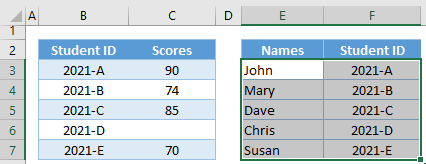
Let’s look at an example where we want to apply conditional formatting based on the result of a VLOOKUP function.

 

Format based on VLOOKUP Comparison

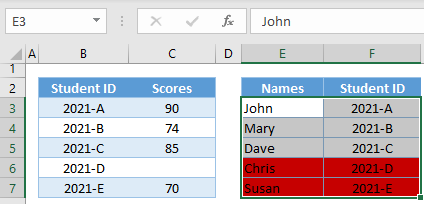
First, we will apply conditional formatting to the table of Names and Student IDs (col E-H) by looking up each student’s grades (Col B-C) and apply RED cell Fill Color if their scores are below 72. The result is shown here, but we will walk through the steps below.

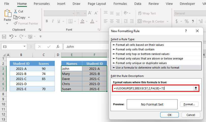
=VLOOKUP($F3,$B$3:$C$7,2,FALSE)<72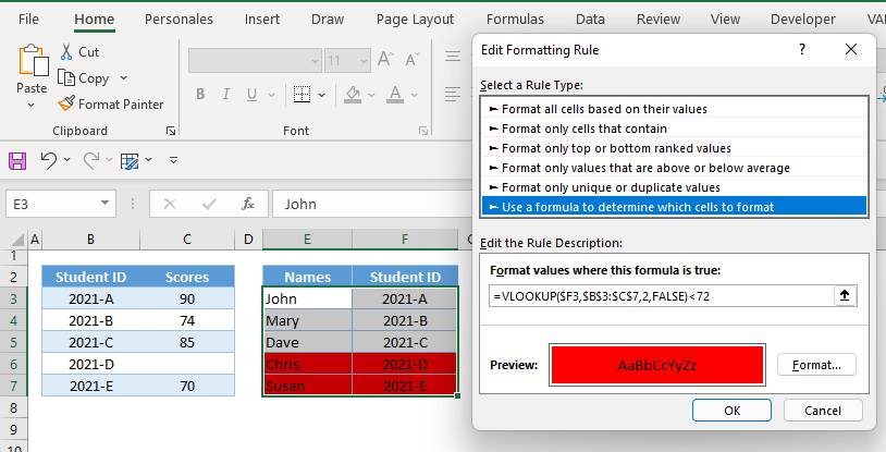

Let’s look at how to apply the above formula in conditional formatting.

Apply Conditional Formatting

1. Highlight the range where the conditional formatting will be applied.

2. In the Ribbon, go to Home Tab > Styles Group > Conditional Formatting > New Rule.

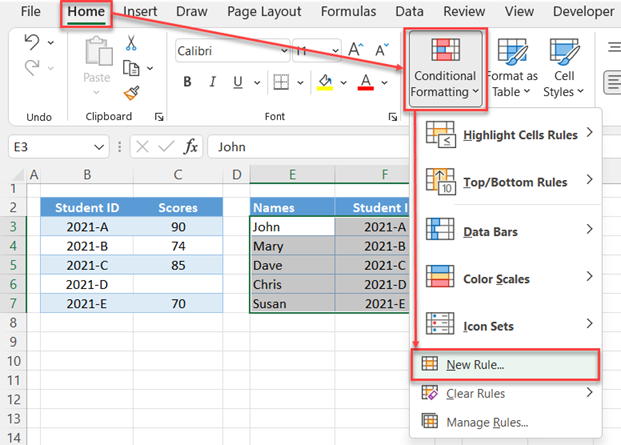
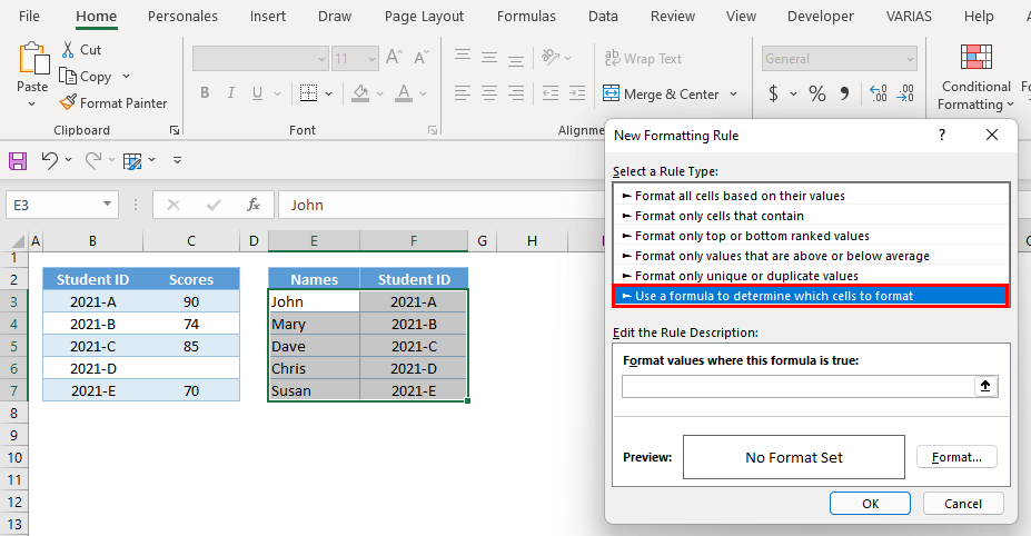
3. In the pop-up menu, select Rule Type: Use a formula to determine which cells to format.

4. In the Formula Bar, input our formula.

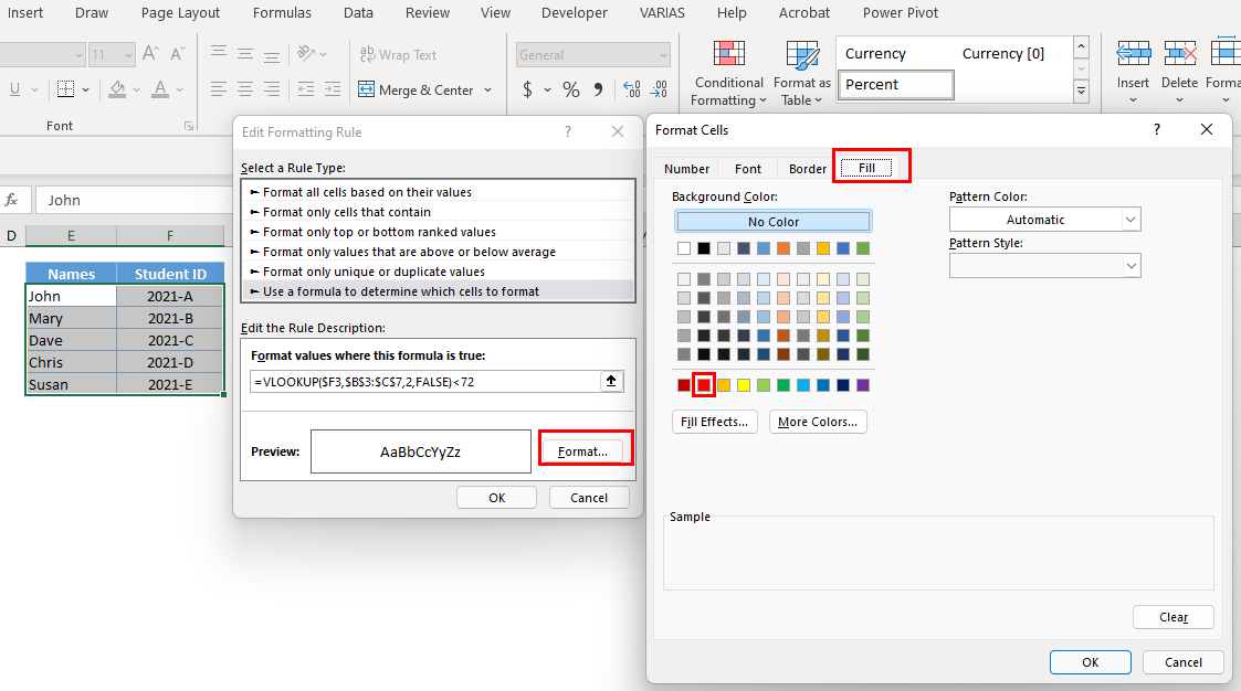
5. Click Format and define your formatting settings. In our case we will choose a RED Fill Color. Click OK.

6. Now click OK and the Conditional Formatting Rule is applied.

 

Now that we know how to apply conditional formatting, let’s walk through the formula.

It can be helpful to start by entering your conditional formatting formula(s) into cells to test that they work as you’d expect. We will do so below.

 

VLOOKUP Function

First, we perform our VLOOKUP.

=VLOOKUP($F3,$B$3:$C$7,2,FALSE)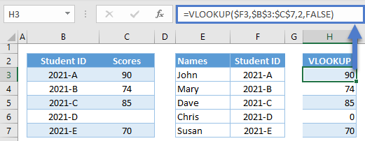

 

We use $s to lock cell references. This is essential to creating a formula that will work for all rows.

Logical Comparison

Next, the results are compared to the set criterion.

=H3<72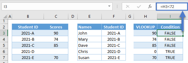

Conditional Formatting will change the cell color for any rows with TRUE.

 

Combining all the formulas together yields our original VLOOKUP formula:

=VLOOKUP($F3,$B$3:$C$7,2,FALSE)<72

 

Format If VLOOKUP is Blank

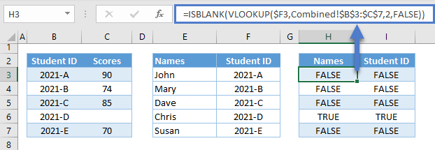
Notice in the previous example, one student did not have a score. We can detect and highlight these cells by adding the ISBLANK Function:

=ISBLANK(VLOOKUP($F3,$B$3:$C$7,2,FALSE))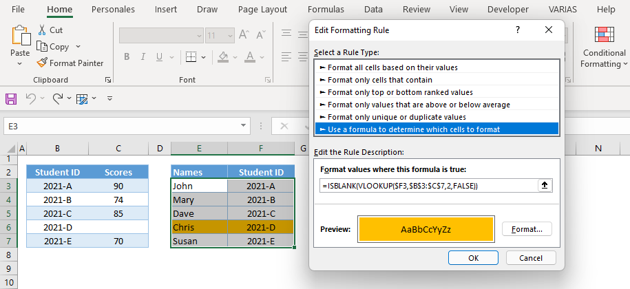

This is how the formula will evaluate:

 

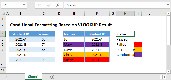
Format If VLOOKUP is within Range of Values

Another common scenario with VLOOKUP is to check if the value is within a given range of values.

To do this, we can use the AND Function together with VLOOKUP:

=AND(VLOOKUP($F3,$B$3:$C$7,2,FALSE)>=72,VLOOKUP($F3,$B$3:$C$7,2,FALSE)<=74)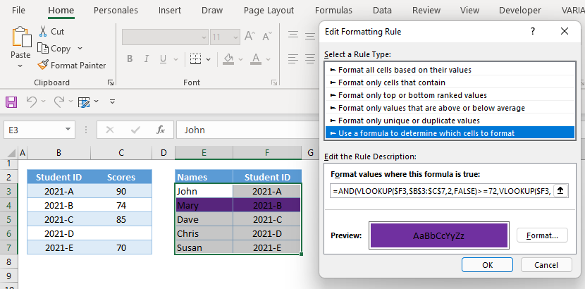

Let’s walk through the formula:

Lower Boundary

First, we check if our VLOOKUP’s output is greater than or equal to a given lower boundary (e.g., 72).

=H3>=72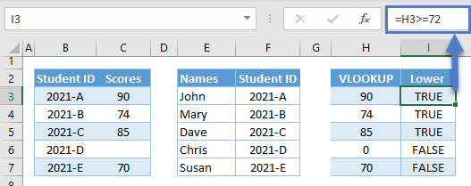

Upper Boundary

Next, we check if that same value is less than or equal to the upper boundary (e.g., 74).

=H3<=74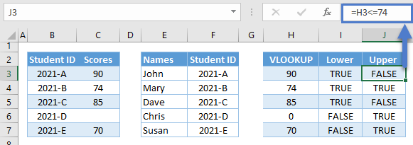

 

AND Function

Finally, we use the AND Function to check if both conditions are TRUE.

=AND(I3,J3)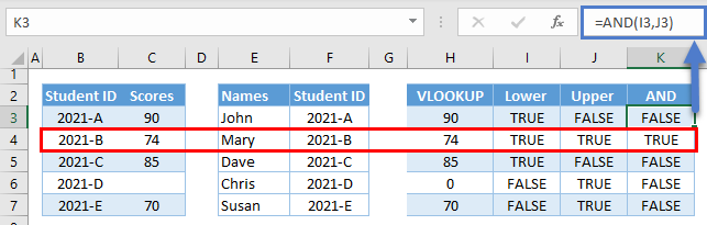

 

Combining the above formulas results in our original formula:

=AND(VLOOKUP($F3,$B$3:$C$7,2,FALSE)>=72,VLOOKUP($F3,$B$3:$C$7,2,FALSE)<=74)

Conditional Formatting – Multiple VLOOKUP Conditions

You can easily add multiple conditional formatting rules:

 

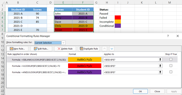
Conditional Formatting rules are applied in order (top to bottom). If Stop if True is checked, then if that condition is met no more formatting rules are tested or applied.

 

In our particular example, the blank VLOOKUP (e.g., ROW 6) satisfies two conditions, red (e.g., <72) and orange (e.g., ISBLANK). Because the ISBLANK rule is applied first and Stop if True is checked, ROW 6 is highlighted ORANGE because the ISBLANK condition is met and subsequent rules are not tested.

 

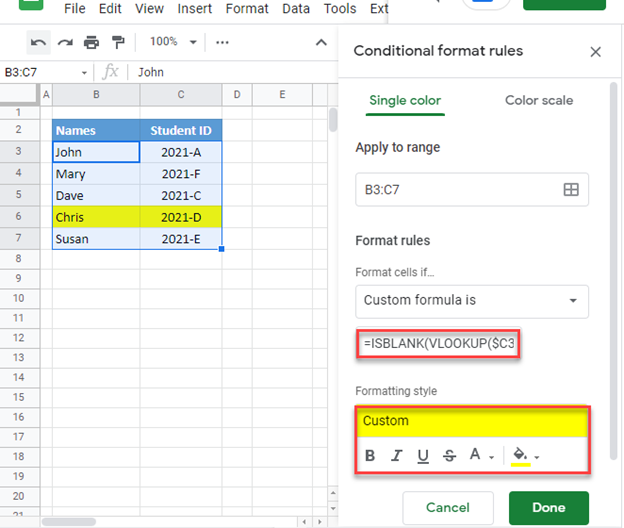
Conditional Formatting based on VLOOKUP Result in Google Sheets

All formulas discussed above work the same way in Google Sheets except if the lookup table is in another sheet. In this instance, we need to use a Named Range or the INDIRECT Function in order to reference ranges from other sheets in conditional formatting.

=ISBLANK(VLOOKUP($C3,INDIRECT("Scores!B3:C7"),2,FALSE))

 

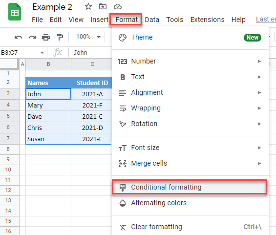
Here are the steps on how to apply conditional formatting in Google Sheets:

1. Highlight the range, and then, go to Format Tab > Conditional Formatting

2. In the sidebar, go to “Format Rules” and select “Custom formula is.”

 

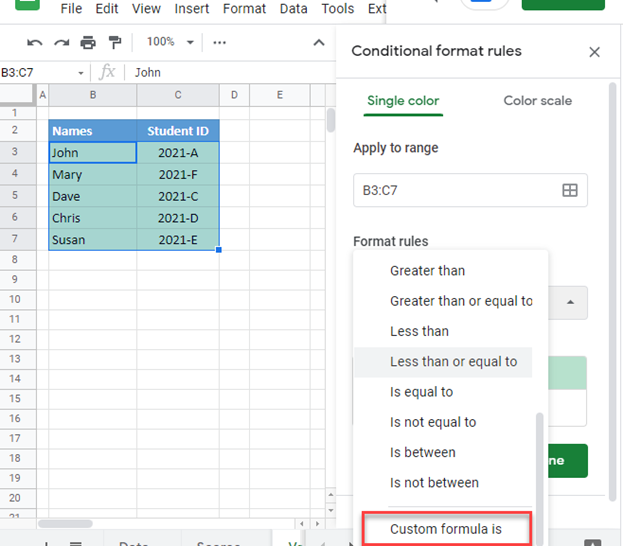
3. Input our formula in the formula bar, and set the formatting style and hit Done: