Use Conditional Formatting With Checkbox in Excel & Google Sheets

This tutorial demonstrates how to use conditional formatting with a checkbox control in Excel and Google Sheets.

 

 

► Click here to jump to the Google Sheets walkthrough.

Conditional Formatting With Checkbox

About Linked Checkboxes

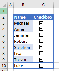
In Excel, you can use a checkbox to control whether a conditional formatting rule is applied. For the following example, you have the data below in Column B and a checkbox for each name in Column C. Each checkbox must be linked to a cell in Column D.

 

 

When you click a checkbox that is linked to a cell, the value in the cell changes to either TRUE or FALSE.

 

 

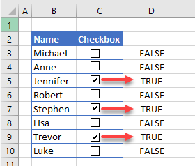
If you do not want to see the TRUE / FALSE values, change the font color to white.

 

 

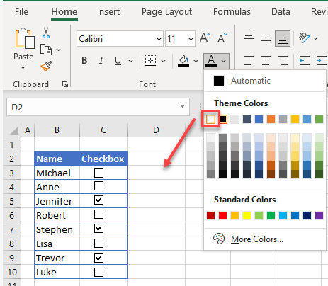
Now, say you want the background color of a name in Column B depending on whether it’s checked (i.e., the value is TRUE).

Change Cell Color With Checkbox

Create a conditional formatting rule for the range containing the names (B3:B10) to add a fill color to a cell when its checkbox is checked. Since the first checkbox is linked to cell D2, this cell’s value is TRUE if the checkbox is checked, and FALSE if it’s unchecked. You’ll use the value of cell D2 as the determinant for the conditional formatting rule.

1. Select the list of names and then, in the Ribbon, go to Home > Conditional Formatting > New Rule.

 

 

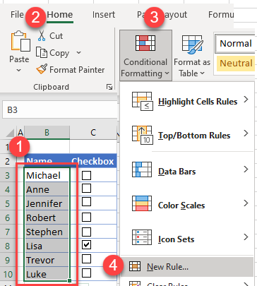
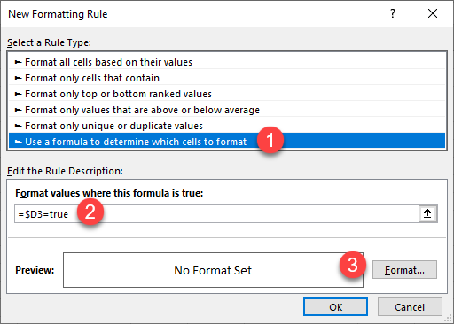
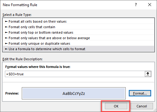
2. From the Rule Type list, (1) choose Use a formula to determine which cells to format. This gives you a formula box under Edit the Rule Description. (2) In the box, enter:

=$D3=TRUE

Ensure that the $ is only on the column reference and not on the row reference. This is known as a mixed reference.
Then (3) click Format.

 

 

3. In the Format Cells window, choose a color (e.g., light blue) and click OK.

 

 

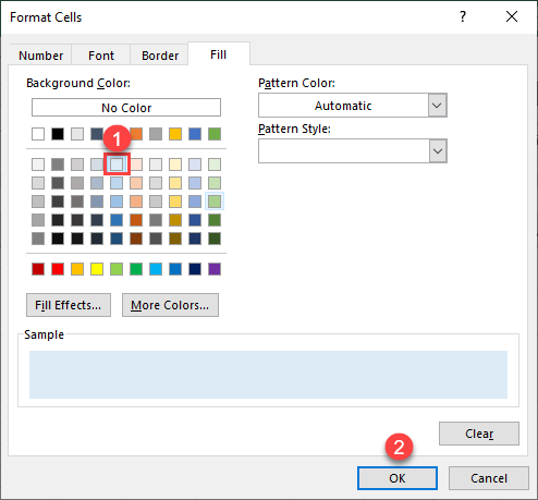
4. That takes you back to the New Formatting Rule window. Click OK.

 

 

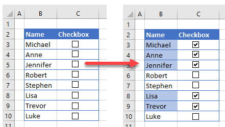
5. Now, when you check the box next to each name, that name cell’s background turns light blue.

 

 

Note: Also learn about using checkboxes with VBA.

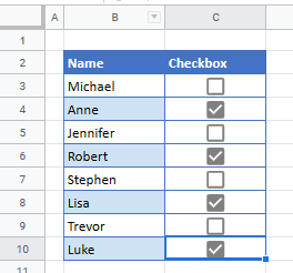
Conditional Formatting With Checkbox in Google Sheets

The process is similar in Google Sheets.

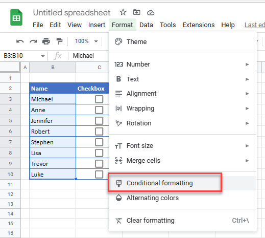
1. Insert a checkbox next to each name in your Google Sheet. You do not have to associate a checkbox in Google Sheets with a cell; linking happens automatically.
2. Select the data range and in the Menu, go to Format > Conditional formatting.

 

 

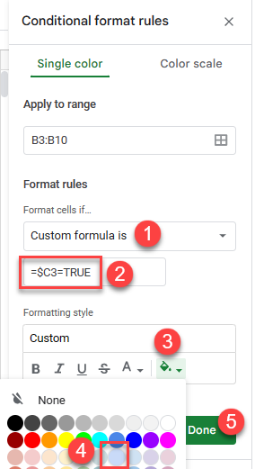
3. In the Conditional format rules window on the right, (1) choose Custom formula is and (2) enter the formula:

=$C3=TRUE

Note that, unlike in Excel, this formula references the cell containing the checkbox.
For the Formatting style, (3) click Fill color, (4) choose the background color (i.e., light blue), and (5) click Done.

 

 

As in Excel, when you check the box next to each name, that name cell’s background turns light blue.