Add a Drop Down List with Color Formatting in Excel & Google Sheets

This tutorial will demonstrate how to add a drop-down list with color formatting in Excel and Google Sheets.

 

 

To create a drop-down list where the background color depends on the text selected, start with Data Validation in Excel, then use Conditional Formatting to amend the background color.

Create a Drop-Down List With Data Validation

 

 

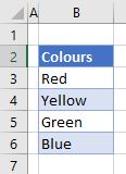
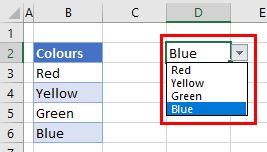
To make a drop-down list from the data contained in a range of cells, start by selecting the cell where you want the drop down to appear.

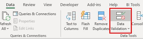
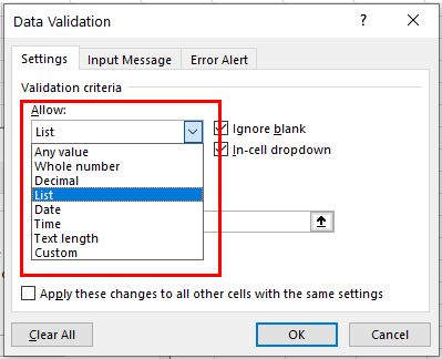
1. In the Ribbon, select Data > Data Tools > Data Validation.

 

 

2. Select List.

 

 

3. Select the range of cells with items as the Source.

 

 

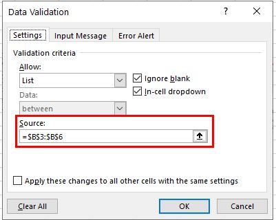
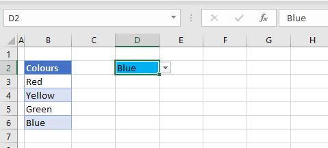
4. Click OK to see the drop-down list in the workbook.

Amend the Background Color With Conditional Formatting

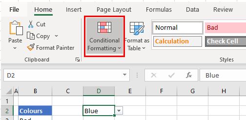
1. Select the cell that contains the drop-down list, and then in the Ribbon, select Home > Styles > Conditional Formatting.

 

 

2. Select New Rule, and then select Format only cells that contain.

 

 

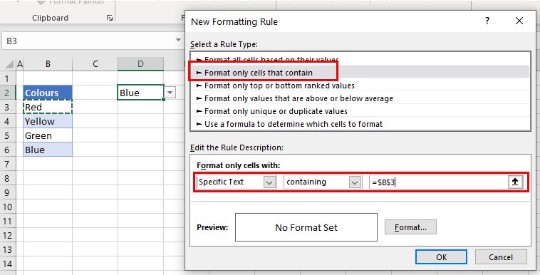
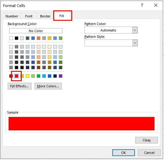
4. Click on the Format… button to set the format. Select the Fill tab and select the color (in this case, red).

 

 

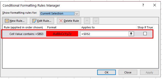
5. Click OK to return to the New Rule screen and then OK to show the Rules Manager.

 

 

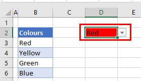
6. Select the drop-down list and change the value to Red to see the result of the Conditional Formatting.

 

 

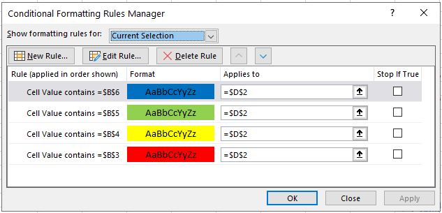
7. Create rules for Yellow, Green, and Blue by following the same steps. The Conditional Formatting Rules Manager should end up having four rules all applying to the cell containing the drop-down list (e.g., D2).

 

 

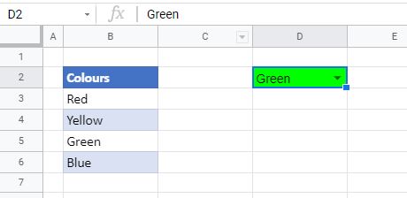
Add a Drop-Down List With Color Formatting in Google Sheets

The process to add a drop-down list with color formatting is much the same in Google Sheets as it is in Excel.

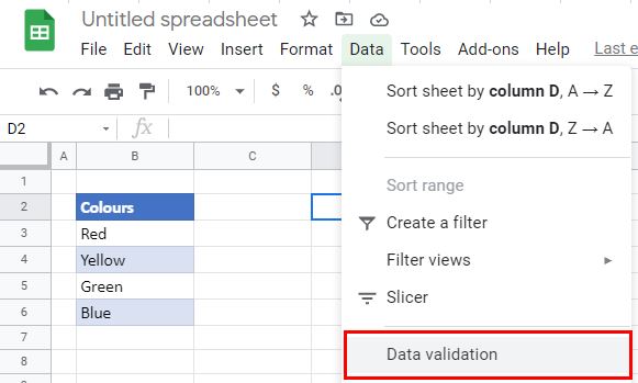
1. In the Menu, select Data > Data validation.

 

 

2. Make sure the Cell range is where the drop-down list should go, and then select the Criteria range (e.g., B3:B6).

 

 

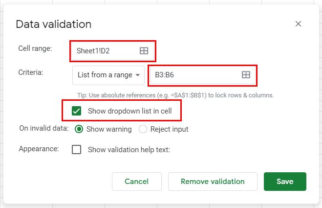
3. Tick Show dropdown list in cell if it not already ticked and then click Save.

 

 

4. With the cell that contains the drop-down list selected, select Format > Conditional formatting from the Menu.

 

 

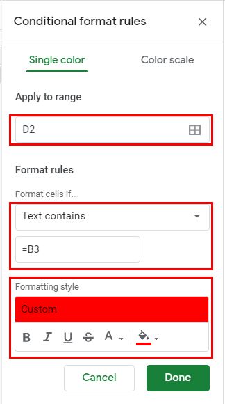
7. Click Add another rule to add the rest of the Conditional Format rules to the drop-down list.

 

 

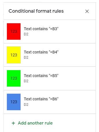
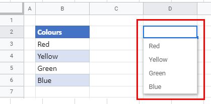
Select a different color from the drop-down list to see the result.