Conditional Formatting Based on Date in Another Cell – Excel & Google Sheets
Written by
Reviewed by
This tutorial will demonstrate how to highlight cells based on a date in another cell using Conditional Formatting in Excel and Google Sheets.
Highlight Cells With Conditional Formatting
To highlight cells that contain a date greater than a date specified in another cell, use a simple formula within Conditional Formatting.
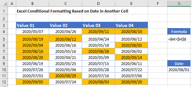
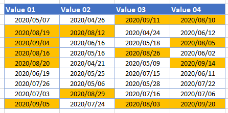
In the following example, you have a table of dates (B4:E12) and want to emphasize which dates are after August 1, 2020. One way to do that is to set another cell (here, G9) to 2020/08/01 and compare each date.
- Select the range where you want to highlight days.
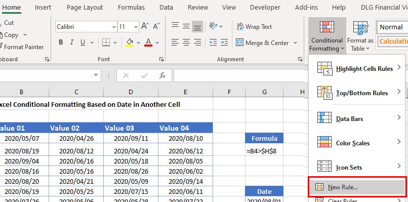
- In the Ribbon, select Home > Conditional Formatting > New Rule.
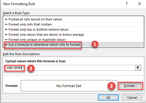
- Select (1) Use a formula to determine which cells to format, and (2) enter the formula:
=B4>$H$8You need to lock the reference to cell H9 by making it absolute. You can do this by typing $ signs around the row and column indicators, or by pressing F4 on the keyboard.
(3) When done, click on Format…
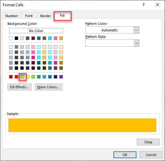
- Select your desired formatting. For this example, apply an orange fill.
- Click OK, then OK again to return to the Conditional Formatting Rules Manager.
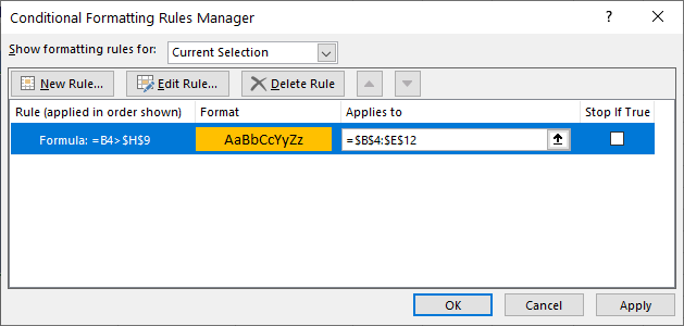
- Click Apply to apply the formatting to your selected range and click Close.
Every cell in the range selected where the date in that cell is greater than the date in cell H8 will have its background color changed to orange.
Highlight Cells with Conditional Formatting in Google Sheets
The process to highlight cells based on the date entered in that cell in Google Sheets is similar to the process in Excel.
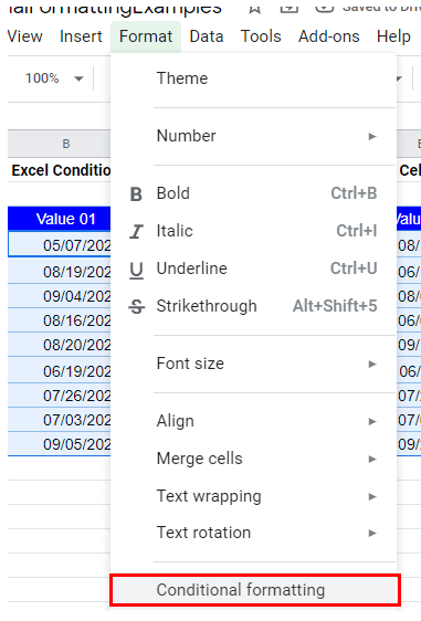
- Highlight the cells you wish to format, and then click on Format > Conditional Formatting.
- The Apply to Range section is automatically filled in.

- From the Format Rules section, select Custom formula is.
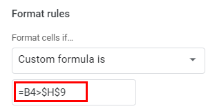
- Select the fill style for the cells that meet the criteria.
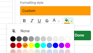
- Click Done to apply the rule.
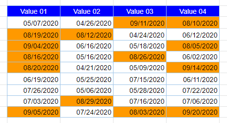
The result is the same: Dates later than Aug 1 are highlighted in orange.
