How to Display Data With Banded Rows in Excel & Google Sheets

This tutorial demonstrates how to display data with banded rows in Excel and Google Sheets.

 

 

Display Banded Rows

Table Formatting

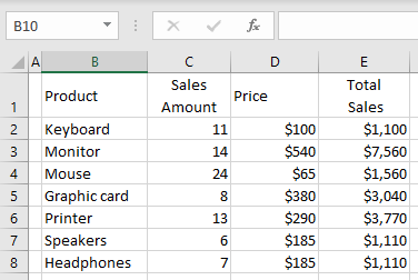
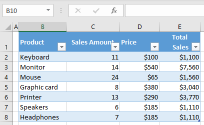
In Excel, you can format your data in banded rows (coloring rows in two alternating colors). One way to do this is by formatting your data as a table. Say you have the following data set in the range B1:E8.

 

 

To display these rows as banded, follow these steps:

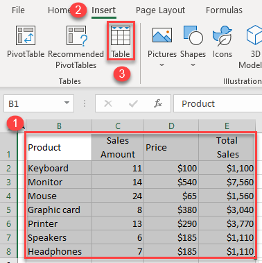
1. First, format your data as a table. Select the data range (here, B1:E8), and in the Ribbon, go to Insert > Table (or use the keyboard shortcut CTRL + T).

 

 

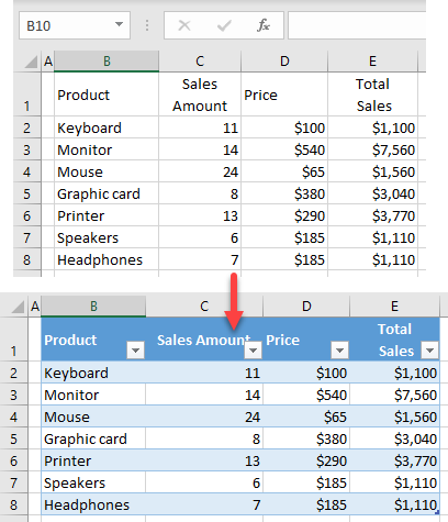
As a result, your data range is converted to a table, and by default, rows are banded in two colors.

 

 

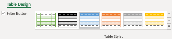
2. If you click on the table, the Table Design tab appears, and when you click on it, you can choose between different table styles with banded rows.

 

 

If you want to keep banded rows and convert the table back to the range, you can use Convert to Range.

For info on using macros with tables, see VBA Tables and ListObjects.

Conditional Formatting

Another way to display banded rows is to use conditional formatting.

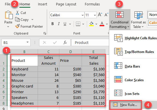
1. Select the data range (B1:E8), and in the Ribbon, go to Home > Conditional Formatting > New Rule…

 

 

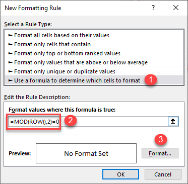
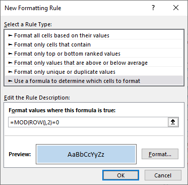
2. In the New Formatting Rule window, choose Use a formula to determine which cells to format, and in the formula box, type:

=MOD(ROW(),2)=0

Then, click Format…
In this formula, the ROW Function returns the number of a row, while the MOD Function returns the remainder of division by two. This way, every even number is formatted according to the conditional formatting rule.

 

 

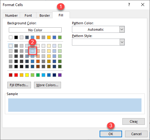
3. In the Format Cells window, go to the Fill tab, choose a color (for example, light blue), and click OK.

 

 

4. Back in the Rule window, you can see the formatting preview. Click OK to finish.

 

 

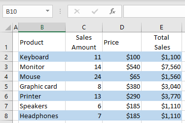
Finally, every second row is now colored in light blue color, as a result of the conditional formatting rule.

 

 

Display Banded Rows in Google Sheets

Alternating Colors

In Google Sheets, you can’t insert a table, but you format cells with alternating colors.

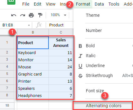
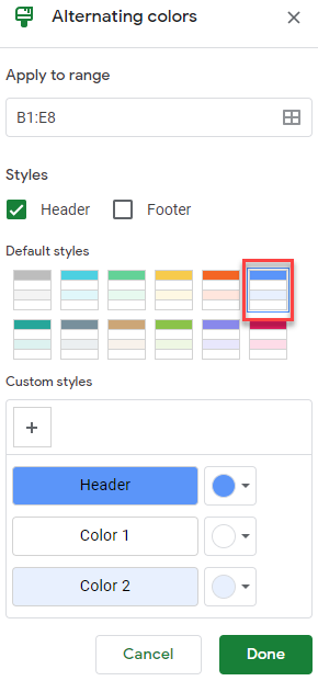
1. Select the data range where you want to display banded rows (B1:E8), and in the Menu, go to Format > Alternating colors.

 

 

2. In the window on the right side, choose a format style (e.g., blue), and click Done. Here, you can also change colors for header and items and make your own custom style.

 

 

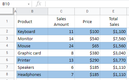
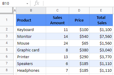
As a result, all rows in the range are now banded.

 

 

Conditional Formatting

Another way to display banded rows is to create a conditional formatting rule, similar to the rule set in Excel above.

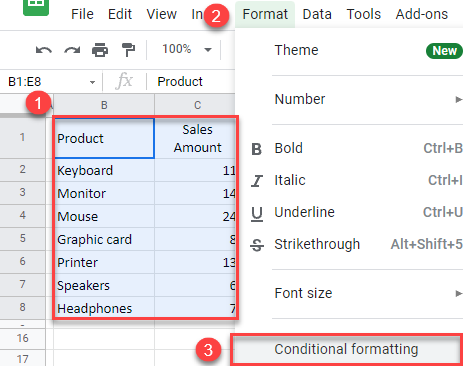
1. Select the data range where you want to display banded rows (B1:E8), and in the Menu, go to Format > Conditional formatting.

 

 

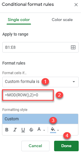
2. In the Conditional format rules window, choose Custom formula is, and enter the formula:

=MOD(ROW(),2)=0

Then, click on the fill color icon to choose a color, and click Done.

 

 

The final output is the same as in Excel, every other row is colored in blue.