MOD Function – Examples in Excel, VBA, Google Sheets
Written by
Reviewed by
Download the example workbook
This tutorial will demonstrate how to use the MOD Function in Excel and Google Sheets to calculate the remainder after dividing.
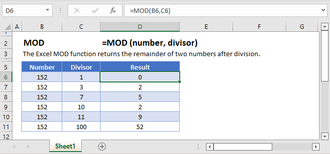
MOD Function Overview
The MOD function returns the remainder, or modulus, of a number after performing division.
However, the MOD function isn’t strictly for helping us with our division problems. It becomes even more powerful for when we want to look for every Nth item in a list, every Nth row, or when we need to generate a repeating pattern.
MOD Basic Math
When you try to divide 13 by 4, you can say the answer is 3 remainder 1. The “1” in this case is specifically known as the modulus (hence the MOD Function name). In a formula then, we could write
=MOD(13, 4)
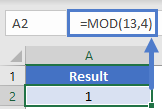
And the output would be 1.
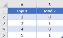
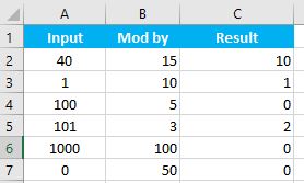
Looking at this table gives some more illustrations of how the input/output of MOD will work.
=MOD(A2,3)
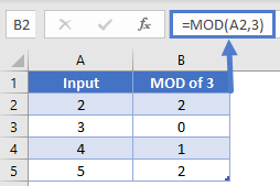
Note that when the input was 3, there was no remainder and thus the output of the formula was 0. Also, in our table we used the ROW Function to generate our values. Much of the power of MOD will be from using the ROW (or COLUMN) function as we’ll see in the following examples.
MOD Sum Every Other Row
Consider this table:
For illustration purposes, the second column has the formula
=MOD(A2, 2)
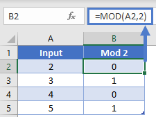 To add all the even rows, you could write a SUMIF Formula and have the criteria look for 0 values in col B. Or, to add all the odd rows, have the criteria be to look for 1 values.
However, we don’t need to create the helper column at all. You can combine the power of MOD within the SUMPRODUCT Function to do it all in one step. Our formula for this would be
=SUMPRODUCT(A2:A5, --(MOD(B2:B2, 2)=0)
Since it’s within SUMPRODUCT, the MOD function will be able to handle our array input. We’ve seen the output already in the helper column, but the array from our MOD in this formula will be {0, 1, 0, 1}. After checking for values that equal 0 applying the double unary, the array will be {1, 0, 1, 0}. The SUMPRODUCT then does it’s magic or multiplying the arrays to produce {2, 0, 4, 0} and then summing to get desired output of 6.
MOD Sum every Nth row
Since a formula of MOD(x, N) will output a 0 at every Nth value, we can use this to help formulas pick and choose which values to use in other functions. Look at this table.
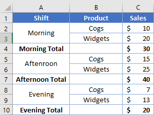
Our goal is to grab the values from each row marked “Total”. Take note that the Total appears every 3rd row, but starting at row 4. Our MOD function will thus use 3 as the 2nd argument, and we need to subtract 1 from the first argument (since 4 -1 = 3). This way the desired rows we want (4, 7, 10) will be multiples of 3 (3, 6, 9). Our formula to sum the desired values will be
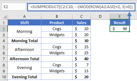
=SUMPRODUCT(C2:C10, --(MOD(ROW(A2:A10)+2, 3)=0))
 The array produced will transform like this:
{2, 3, 4, 5, 6, 7, 8, 9, 10}
{1, 2, 3, 4, 5, 6, 7, 8, 9}
{1, 2, 0, 1, 2, 0, 1, 2, 0}
{False, False, True, False, False, True, False, False, True}
{0, 0, 1, 0, 0, 1, 0, 0, 1}
Our SUMPRODUCT’s criteria array is now setup how we need to grab every 3rd value, and we’ll get our desired result of $90.
MOD Sum on Columns
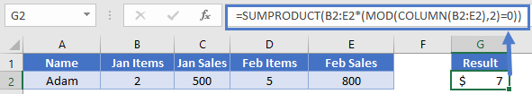
We’ve been using examples so far that go vertically and use ROW, but you can also go horizontally with the COLUMN function. Consider this layout:
![]()
We want to sum up all the items. Our formula for this could be
=SUMPRODUCT(B2:E2*(MOD(COLUMN(B2:E2), 2)=0)
In this case, we’re setup to grab every 2nd column within our range, so the SUMPRODUCT will only retain non-zero values for columns B & D. For reference’s here’s a table showing column numbers and their corresponding value after taking MOD 2.
Highlight every Nth row
Another common use of the MOD function is to highlight every Nth row. The general form for this will be:
=MOD(ROW() ± Offset, N)=0
Where N is the number of rows between each highlighted row (I.e., to highlight every 3rd row, N = 3), and Offset is optionally the number we need to add or subtract to get our first highlighted row to align with N (I.e., to highlight every 3rd row but start at row 5, we’d need to subtract 2 since 5 -2 = 3). Note that with the ROW function, by omitting any arguments, it will return the row number from cell the formula is in.
Let’s use our table from before:
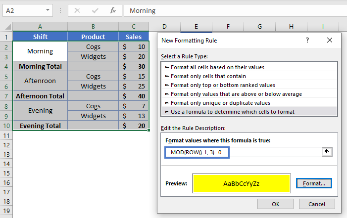
To apply a highlight to all the Total rows, we’ll create a new Conditional Formatting rule with a formula of
=MOD(ROW()-1, 3)=0
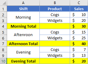
When the conditional formatting applies this formula, row 2 will see
=MOD(2-1, 3)=0
=MOD(1, 3) = 0
=1=0
=False
Row 3 will experience a similar output, but then row 4 will see
=MOD(4-1, 3)=0
=MOD(3, 3) = 0
=0=0
=True
Highlight Integers or Even numbers
Rather than highlighting specific rows, you could also check the actual values within the cells. This could be useful for when you want to find numbers that are multiples of N. For instance, to find multiples of 3 your conditional format formula would be
=MOD(A2, 3)=0
Up to this point, we’ve been dealing with whole numbers. You can have an input of a decimal (e.g. 1.234) however and then divide by 1 to get only the decimal portion (e.g. 0.234). This formula looks like
=MOD(A2, 1)
Knowing that, to highlight only integers the conditional format formula would be
=MOD(A2, 1)=0
Concatenate every N Cells
We’ve previously been using MOD to tell the computer when to grab at value at every Nth item. You could also have it be used to trigger a larger formula to be executed. Consider this layout:
We want to concatenate the names together, but only on every 3rd row starting on row 2. The formula used for this is
=IF(MOD(ROW()+1, 3)=0, CONCATENATE(A2," ", A3," ", A4), "")
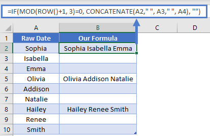 Our MOD function is what’s acting as the criteria for the overall IF function. In this example, we added 1 to our ROW, because we’re starting at row 2 (2 + 1 = 3). When the MOD’s output is 0, the formula does the concatenation. Otherwise, it just returns blank.
Count Even / Odd Values
If you’ve ever needed to count how many even or odd values are in a range, you’ll know that COUNTIF doesn’t have the ability to do this. We can do it with MOD and SUMPRODUCT though. Let’s look at this table:
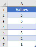
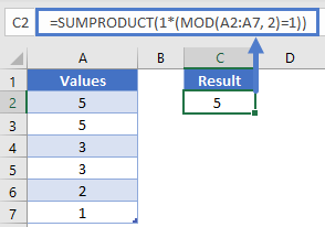
The formula we’ll use to find the odd values will be
=SUMPRODUCT(1*(MOD(A2:A7, 2)=1))
 Rather than loading in some row numbers, our MOD is going to load in the actual cells’ values into the array. The overall transformation will then progress like so:
{5, 5, 3, 3, 2, 1}
{1, 1, 1, 1, 0, 1}                            <- Took the mod of 2
{ True, True, True, True, False, True }       <- Checked if value was 0
{1, 1, 1, 1, 0, 1}                            <- Multiplied by 1 to convert from True/False to 1/0
The SUMPRODUCT then adds up the values in our array, giving desired answer of: 5.
Repeating Pattern
All the previous examples have been checking the output of MOD for a value. You can also use MOD to generate a repeating pattern of numbers, which can in turn be very helpful.
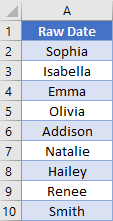
First, let’s say that we had a list of items we want repeated.

You could try and manually copy & paste however many times you need, but that would get tedious. Instead, we’ll want to use the INDEX Function to retrieve our values. For the INDEX to work, we need the row argument to be a sequence of numbers that goes {1, 2, 3, 1, 2, 3, 1, etc.}. We can accomplish this using MOD.
First, we’ll start with just the ROW function. If you start with
=ROW(A1)
And then copy this downwards, you get the basic number sequence of {1, 2, 3, 4, 5, 6, …}. If we applied the MOD function with 3 as the divisor,
=MOD(ROW(A1), 3)
we’d get {1, 2, 0, 1, 2, 0, …}. We see that we’ve got a repeating pattern of “0, 1, 2”, but the first series is missing the initial 0. To fix this, back up a step and subtract 1 from the row number. This will change our starting sequence to {0, 1, 2, 3, 4, 5, …}
=MOD(ROW(A1)-1, 3)
And after it comes out of the MOD, we have {0, 1, 2, 0, 1, 2, …}. This is getting close to what we need. The last step is to add 1 to the array.
=MOD(ROW(A1)-1, 3)+1
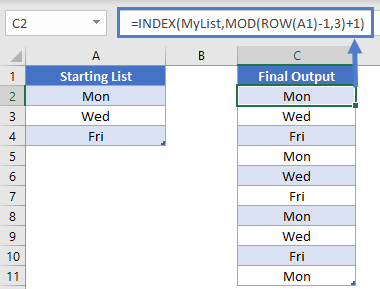
Which now produces a number sequence of {1, 2, 3, 1, 2, 3, …}. This is our desired sequence! Plugging it into an INDEX function, we get our formula of
=INDEX(MyList, MOD(ROW(A1)-1, 3)+1)
The output will now look like this:
MOD Examples in VBA
You can also use the MOD Function in VBA.
Within VBA, MOD is an operator (just like plus, minus, multiplication and division operators). So, executing the following VBA statements
Range("C2") = Range("A2") Mod Range("B2")
Range("C3") = Range("A3") Mod Range("B3")
Range("C4") = Range("A4") Mod Range("B4")
Range("C5") = Range("A5") Mod Range("B5")
Range("C6") = Range("A6") Mod Range("B6")
Range("C7") = Range("A7") Mod Range("B7")
will produce the following results
For the function arguments (known_y’s, etc.), you can either enter them directly into the function, or define variables to use instead.
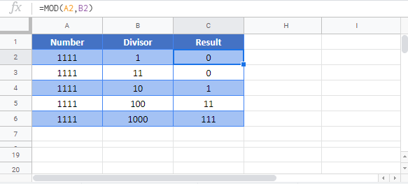
Google Sheets MOD Function
The MOD Function works exactly the same in Google Sheets as in Excel: