This tutorial demonstrates how to use the Excel IF Function in Excel to create If Then Statements.

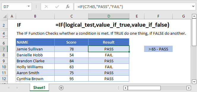
IF Function Overview

The IF Function Checks whether a condition is met. If TRUE do one thing, if FALSE do another.

To use the IF Excel Worksheet Function, select a cell and type:

(Notice how the formula inputs appear)

IF function Syntax and inputs:

=IF(logical_test,value_if_true,value_if_false)

logical_test – Logical expression. Example: A1 > 4.

value_if_true – Value or Calculation to perform if logical expression is TRUE.

value_if_false – Value or Calculation to perform if logical expression is FALSE.

 

What is the IF Function?

IF is a “conditional” function. This means you define a logical test, and it will return one value if that test evaluates as true, and a different value if it is false

 

How to Use the IF Function

Here’s a very basic example so you can see what I mean. Try typing the following into Excel:

=IF( 2 + 2 = 4,"It’s true", "It’s false!")

Since 2 + 2 does in fact equal 4, Excel will return “It’s true!”. If we used this:

=IF( 2 + 2 = 5,"It’s true", "It’s false!")

Now Excel will return “It’s false!”, because 2 + 2 does not equal 5.

Here’s how you might use IF in a spreadsheet.

=IF(C4-D4>0,C4-D4,0)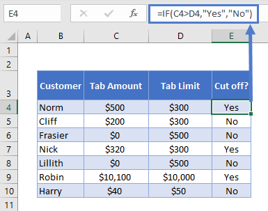

You run a sports bar and you set individual tab limits for different customers. You’ve set up this spreadsheet to check if each customer is over their limit, in which case you’ll cut them off until they pay their tab.

You check if C4-D4 (their current tab amount minus their limit), is greater than 0. This is your logical test. If this is true, IF returns “Yes” – you should cut them off. If this is false, IF returns “No” – you let them keep drinking.

 

What IF can return

Above we returned a text string, “Yes” or “No”. But you can also return numbers, or even other formulas.

Let’s say some of your customers are running up big tabs. To discourage this, you’re going to start charging interest on customers who go over their limit.

You can use IF for that:

=IF(C4>D4,C4*0.03,0)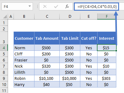

If the tab is higher than the limit, return the tab multiplied by 0.03, which returns 3% of the tab. Otherwise, return 0: they aren’t over their tab, so you won’t charge interest.

 

Using IF with AND

You can combine IF with Excel’s AND function <<link>>. You use this in the logical test, which enables you to specify two or more conditions to test. Excel will only return TRUE if ALL of the tests are true.

So, you implemented your interest rate. But some of your regulars are complaining. They’ve always paid their tabs in the past, why are you cracking down on them now? You come up with a solution: you won’t charge interest to certain trusted customers.

You make a new column to your spreadsheet to identify trusted customers, and update your IF statement with an AND function:

=IF(AND(C4>D4, F4="No"),C4*0.03,0)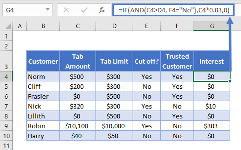

Let’s look at the AND part separately:

AND(C4>D4, F4="No")

Note the two conditions:

• C4>D4: checking if they’re over their tab limit, as before
• F4=”No”: this is the new bit, checking if they are not a trusted customer

So now we only return the interest rate if the customer is over their tab, AND we have “No” in the trusted customer column. Your regulars are happy again.

Read more on the main page for the Excel AND Function <<link>>.

 

Using IF with OR

OR is another of Excel’s logical functions. Like AND, it enables you to define more than one condition. But unlike AND, it will return TRUE if ANY of the tests you define are true.

Maybe customers being over their tab is not the only reason you’d cut them off. Maybe you give some people a temporary ban for other reasons, gambling on the premises perhaps.

So you add a new column to identify banned customers, and update your “Cut off?” column with an OR test:

=IF(OR(C4>D4,E4="Yes"),"Yes","No")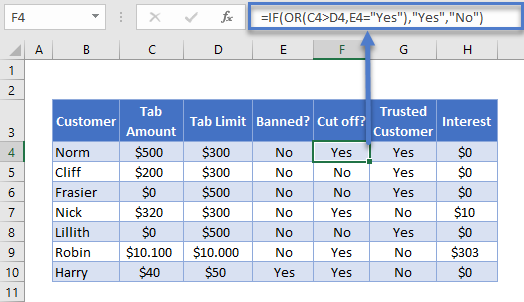

Looking just at the OR part:

OR(C4>D4,E4="Yes")

There are two conditions:

• C4>D4: checking if they’re over their tab limit
• F4=”Yes”: the new part, checking if they are currently banned

This will evaluate to true if they are over their tab, or if there is a “Yes” in column E. As you can see, Harry is cut off now, even though he’s not over his tab limit.

Read more on the main page for the Excel OR Function <<link>>.

Using IF with XOR

XOR is another logical function, which returns the “Exclusive Or”. This is a little less intuitive than the previous ones we’ve discussed.

In simple cases, you define two conditions, and XOR will return:

• TRUE if either argument is true (same as a normal OR)
• FALSE if both arguments are true
• FALSE if both arguments are false

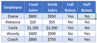
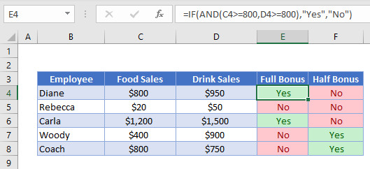
An example might make this clearer. Imagine you want to start giving monthly bonuses to your staff :

• If they sell over $800 in food, or over $800 in drinks, you’ll give them a half bonus
• If they sell over $800 in both, you’ll give them a full bonus
• If they sell under $800 in both, they don’t get any bonus.

You already know how to work out if they get the full bonus. You’d just use IF with AND, as described earlier.

=IF(AND(C4>800,D4>800),"Yes","No")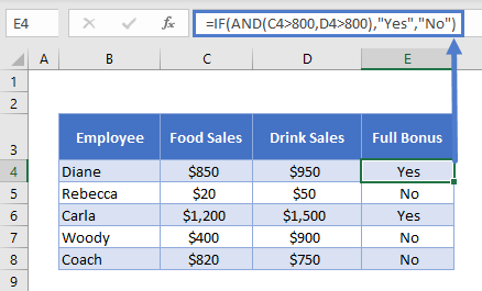

But how would you work out who gets the half bonus? That’s where XOR comes in:

=IF(XOR(C4>=800,D4>=800),"Yes","No")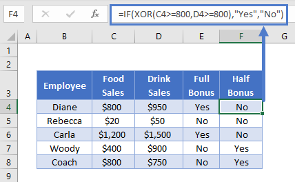

As you can see, Woody’s drink sales were over $800, but not food sales. So he gets the half bonus. The reverse is true for Coach. Diane and Carla sold more than $800 for both, so they don’t get a half bonus (both arguments are TRUE), and Rebecca made under the threshold for both (both arguments FALSE), so the formula again returns “No”.

Read more on the main page for the Excel XOR Function <<link>>.

Using IF with NOT

NOT is yet another of Excel’s logical functions, which is very commonly used with IF.

NOT reverses the outcome of a logical test. In other words, it checks whether a condition has not been met.

You can use it with IF like this:

=IF(AND(C3>=1985,NOT(D3="Steven Spielberg")),"Watch", "Don’t Watch")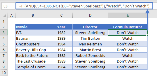

Here we have a table with data on some 1980s movies. We want to identify movies released on or after 1985, that were not directed by Steven Spielberg.

Because NOT is nested within an AND Function, Excel will evaluate that first. It will then use the result as part of the AND.

Read more on the main page on the Excel NOT Function <<link>>.

Nested IF Statements

You can also return an IF statement within your IF statement. This enables you to make more complex calculations.

Let’s go back to our customers table. Imagine you want to classify customers based on their debt level to you:

• $0: None
• Up to $500: Low
• $500 to $1000: Medium
• Over $1000: High

You can do this by “nesting” IF statements:

=IF(C4=0,"None",IF(C4<=500,"Low",IF(C4<=1000,"Medium",IF(C4>1000,"High"))))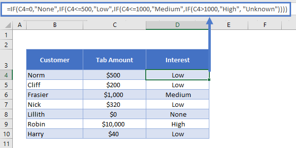

It’s easier to understand if you put the IF statements on separate lines (ALT + ENTER on Windows, CTRL + COMMAND + ENTER on Macs):

=
IF(C4=0,"None",
IF(C4<=500,"Low",
IF(C4<=1000,"Medium",
IF(C4>1000,"High", "Unknown"))))

IF C4 is 0, we return “None”. Otherwise, we move to the next IF statement. IF C4 is equal to or less than 500, we return “Low”. Otherwise, we move on to the next IF statement… and so on.

Simplifying Complex IF Statements with Helper Columns

If you have multiple nested IF statements, and you’re throwing in logic functions too, your formulas can become very hard to read, test, and update.

This is especially important to keep in mind if other people will be using the spreadsheet. What makes sense in your head, might not be so obvious to others.

Helper columns are a great way around this issue.

You’re an analyst in the finance department of a large corporation. You’ve been asked to create a spreadsheet that checks whether each employee is eligible for the company pension.

Here’s the criteria:

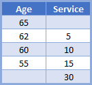
So if you’re under the age of 55, you need to have 30 years’ service under your belt to be eligible. If you’re aged 55 to 59, you need 15 years’ service. And so on, up to age 65, where you’re eligible no matter how long you’ve worked there.

You could use a single, complex IF statement to solve this problem:

=IF(OR(F4>=65,AND(F4>=62,G4>=5),AND(F4>=60,G4>=10),AND(F4>=55,G4>=15),G4>30),"Eligible","Not Eligible")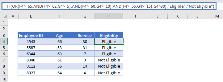

Whew! Kinda hard to get your head around that, isn’t it?

 

A better approach might be to use helper columns. We have five logical tests here, corresponding to each row in the criteria table. This is easier to see if we add line breaks to the formula, as we discussed earlier:

=IF(
OR(
F4>=65,
AND(F4>=62,G4>=5),
AND(F4>=60,G4>=10),
AND(F4>=55,G4>=15),
G4>30
),"Eligible","Not Eligible")

So, we can split these five tests into separate columns, and then simply check whether any one of them is true:

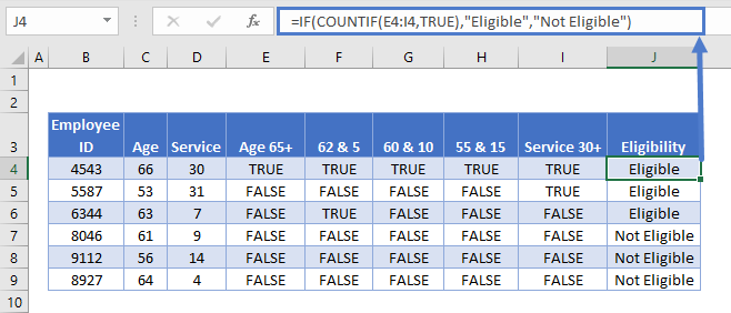
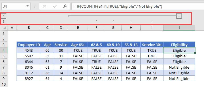
Each column in the table from E to I holds each of our criteria separately. Then in J4 we have the following formula:

=IF(COUNTIF(E4:I4,TRUE),"Eligible","Not Eligible")

Here we have an IF statement, and the logical test uses COUNTIF <<link>> to count the number of cells within E4:I4 that contain TRUE.

If COUNTIF doesn’t find a TRUE value, it will return 0, which IF interprets as FALSE, so the IF returns “Not Eligible”.

If COUNTIF does find any TRUE values, it will return the number of them. IF interprets any number other than 0 as TRUE, so it returns “Eligible”.

Splitting out the logical tests in this way makes the formula easier to read, and if something’s going wrong with it, it’s much easier to spot where the mistake is.

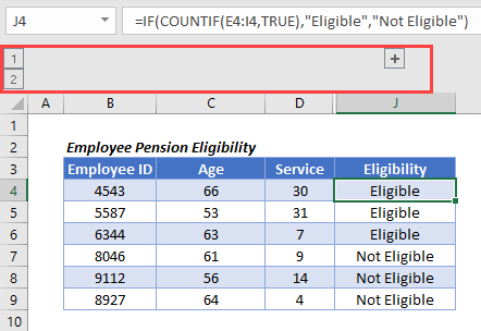
Using Grouping to Hide Helper Columns

Helper columns make the formula easier to manage, but once you’ve got them in place and you know they are working correctly, they often just take up space on your spreadsheet without adding any useful information.

You could hide the columns, but this can lead to problems because hidden columns are hard to detect, unless you look closely at the column headers.

A better option is grouping.

Select the columns you want to group, in our case E:I. Then press ALT + SHIFT + RIGHT ARROW on Windows, or COMMAND + SHIFT + K on Mac. You can also go to the “Data” tab on the ribbon and select “Group” from the “Outline” section.

You’ll see the group displayed above the column headers, like this:

Then simply press the “-“ button to hide the columns:

The IFS Function

Nested IF statements are very useful when you need to perform more complex logical comparisons, and you need to do it in one cell. However, they can get complicated as they get longer, and they can be hard to read and update on your screen.

From Excel 2019 and Excel 365, Microsoft introduced another function, IFS, to help make this a bit easier to manage. The nested IF example above could be achieved with IFS like this:

=IFS(
C4=0,"None",
C4<=500,"Low",
C4<=1000,"Medium",
C4>1000,"High",
TRUE, "Unknown",
)

You can read all about it on the main page for the Excel IFS Function <<link>>.

 

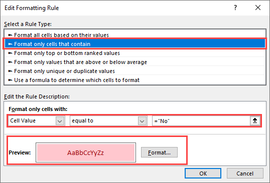
Using IF with Conditional Formatting

Excel’s conditional formatting feature enables you to format a cell in different ways depending on its contents. Since the IF returns different values based on our logical test, we might want to use conditional formatting to make these different values easier to see.

 

So let’s go back to our staff bonus table from earlier.

 

We’re returning “Yes” or “No” depending on what bonus we want to give. This tells us what we need to know, but the information doesn’t jump out at us. Let’s try to fix that.

 

Here’s how you’d do it:

 

• Select the cell range containing your IF statements. In our case that’s E4:F8.
• Click “Conditional Formatting” on the “Styles” section of the “Home” tab on the ribbon.
• Click “Highlight Cells Rules” and then “Equal to”.
• Type “Yes” (or whatever return value you need) into the first box, and then choose the formatting you want from the second box. (I’ll choose green for this).
• Repeat for all your return values (I’ll also set “No” values to red)

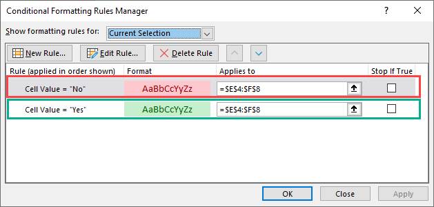
Here’s the result:

 

Using IF in Array Formulas

An array is a range of values, and in Excel arrays are represented as comma separated values enclosed in braces, such as:

{1,2,3,4,5}

The beauty of arrays, is that they enable you to perform a calculation on each value in the range, and then return the result. For example, the SUMPRODUCT Function takes two arrays, multiplies them together, and sums the results.

So this formula:

=SUMPRODUCT({1,2,3},{4,5,6})

…returns 32. Why? Let’s work it through:

1 * 4 = 4
2 * 5 = 10
3 * 6 = 18

4 + 10 + 18 = 32

We can bring an IF statement into this picture, so that each of these multiplications only happens if a logical test returns true.

For example, take this data:

https://www.automateexcel.com/excel/wp-content/uploads/2020/07/SUMPRODUCT-Example-Range.png?ezimgfmt=ng:webp/ngcb20

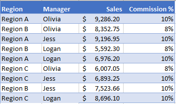
If you wanted to calculate the total commission for each sales manager, you’d use the following:

=SUMPRODUCT(IF($C$2:$C$10=$G2,$D$2:$D$10*$E$2:$E$10))

Note: In Excel 2019 and earlier, you have to press CTRL + SHIFT + ENTER to turn this into an array formula.

We’d end up with something like this:

https://www.automateexcel.com/excel/wp-content/uploads/2020/07/SUMPRODUCTS-IF-Results-Table.png?ezimgfmt=rs:198×95/rscb20/ng:webp/ngcb20

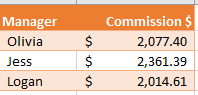
Breaking this down, the “Manager” column is column C, and in this example, Olivia’s name is in G2.

So the logical test is:

$C$2:$C$10=$G2

In English, if the name in column C is equal to what’s in G2 (“Olivia”), DO multiply the values in columns D and E for that row. Otherwise, don’t multiply them. Then, sum all the results.

You can learn more about this formula on the main page for the SUMPRODUCT IF Formula <<llink>>.

 

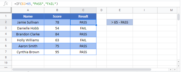
IF in Google Sheets

The IF Function works exactly the same in Google Sheets as in Excel:

Additional Notes

Use the IF Function to test if a condition is TRUE. If the condition is TRUE then do one thing. If it’s FALSE then do another. The condition must be a logical expression (ex: a1 >5), a reference to a cell containing TRUE or FALSE, or an array containing all logical values.

The IF Function can only test one condition at a time. However, you can “nest” other logical functions within the IF condition to test multiple conditions at once:

=if(AND(a1>0,a2>0),TRUE,FALSE)
=if(OR(a1>0,a2>0),TRUE,FALSE)
=if(XOR(a1>0,a2>0),TRUE,FALSE)
OR Functions test if one or more conditions are met.
AND Functions test if all conditions are met.
XOR Functions test if one and only one condition are met.

You can also “nest” an IF Function within an IF Function:

=if(a1<0,if(a2<0,"Both","only 1"),"only one")

Now for some concrete examples of how the IF function works in practice:

1. Start a New Work book.

2. In Cell A1 enter the value 10 (and press Enter)

3. Then in Cell B1 enter the following formula:

=IF(A1 > 5,"BIGGER THAN 5","LESS THAN 5")

4. The screen should look like this now:

5. If you’ve entered the formula correctly, you will see the message “Bigger than 5” appear in cell B1.

6. The formula you’ve entered in Cell B1 performs the test “A1> 5” i.e it checks if the value in Cell A1 is greater than 5.  Currently the value in Cell A1 is 10 – so the condition is TRUE and the message “BIGGER THAN 5” appears

7. If we now change the value in cell A1 to 2:

Thtn the message in cell B2 is now “LESS THAN 5” as the condition is FALSE.

8. You can keep changing the value in cell A1 and the message in cell B2 will adjust accordingly.

9. Of course there are situations where the condition could give mischievous results:

•    What happens if we enter the Value 5 in Cell A1 ?

•    What about if we leave Cell A1 blank ?

•    What about if we put some text in Cell A1 e.g  the phrase DOG

More on the Excel IF Function

We will now look at the IF function in more detail. It can be used to analyse large quantities of data very easily.

Imagine that you are a Area Sales Manager and have a Sales Team. You could record the total Sales that each person makes in a simple Excel Spreadsheet:

Suppose that the criteria for a bonus was that the Sales made by that person exceeded £ 40,000. You could just “eye-ball” the data and determine that only Anton , Newton and Monique met the target.

This is quite easy when you’ve got just a handful of names. However if you’ve got several then there is scope for error. Fortunately by using Excel’s IF function it can be done much faster and safer.

Set up a new workbook and type in the data as per above. Then in cell D4 type in the following formula :-

=IF(C4>40000,"BONUS PAYABLE","NO BONUS")

so that you have:

Note how Excel shows the structure of the IF formula – which is a useful aide memoire.

Having typed in the formula press ENTER and you see it evaluate for the first row:

The formula has been evaluated for Martin – as he earned less than £ 40,000 he isn’t entitled to any bonus.

And then we drag the formulae down by clicking the bottom right hand corner and dragging down we can determine whether or each person is entitled to a bonus:

And we see that Excel has determined which of the Sales People are entitled to a bonus.

Return to the List of all Functions in Excel

VBA IF Statements

You can also use If Statements in VBA. Click the link to learn more, but here is a simple example:

Sub Test_IF ()

If Range("a1").Value < 0 then
  Range("b1").Value = "Negative"
End If

End If

This code will test if a cell value is negative. If so, it will write “negative” in the next cell.