How to Change Table Style in Excel & Google Sheets

This tutorial demonstrates how to change table styles in Excel and Google Sheets.

 

 

Change Excel Table Style

If your data is formatted as a table in Excel, you can access the Table Design tab on the Ribbon.

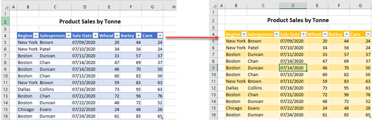
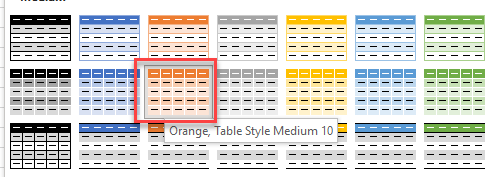
1. Select the table, and then in the Ribbon, go to Table Design > Table Styles. Scroll to show alternative styles in the style box, and then click on the Style you want.

 

 

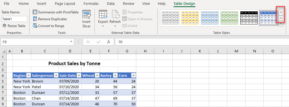
2. Alternatively, to see more styles, click on the More button (the bottom down arrow).

 

 

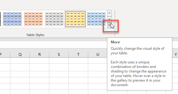
3. This brings up a list of all available styles.

 

 

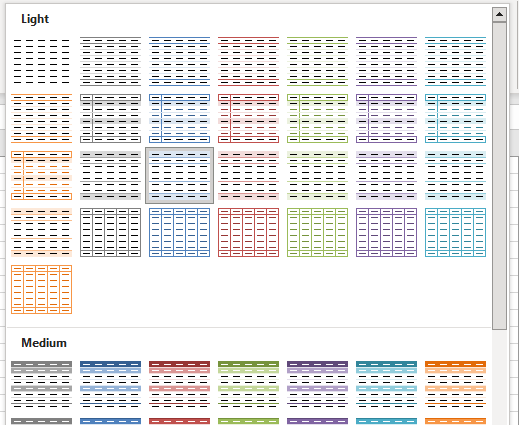
4. Select the one you want to apply it to your table.

 

 

Create Custom Style

You can also create a custom style.

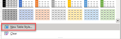
1. At the bottom of the list of styles, click New Table Style…

 

 

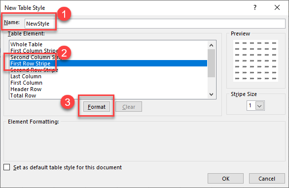
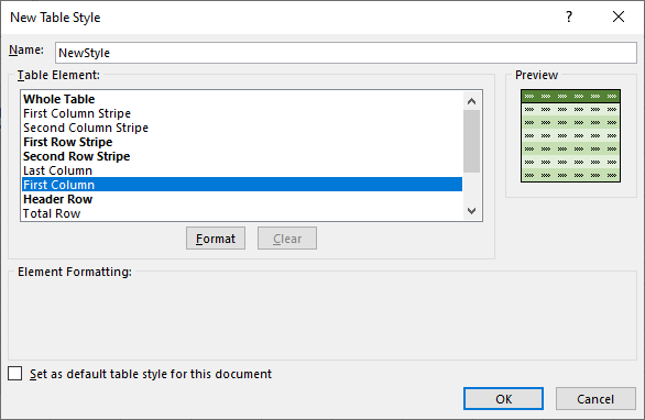
2. In the Name field, type a new name for your style. Then from the Table Element list, choose the property to format. Finally, click Format.

 

 

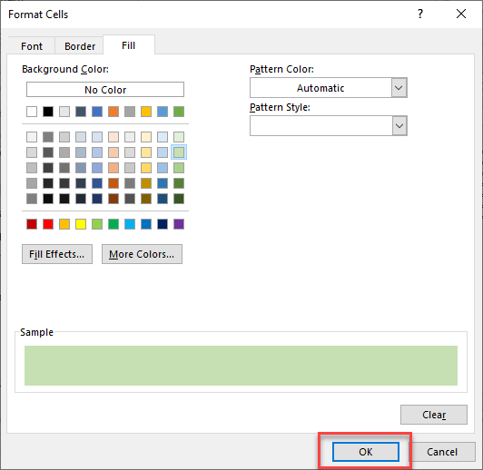
3. Adjust the Font, Border, and Fill. Then click OK to close the Format Cells dialog box.

 

 

4. Notice that in the Table Element list, the elements that you formatted are now bolded. A preview of your style is shown on the right side of the New Table Style box. Click OK to add your New Style to the list.

 

 

5. Click in the table styles box and choose a custom style to apply.

 

 

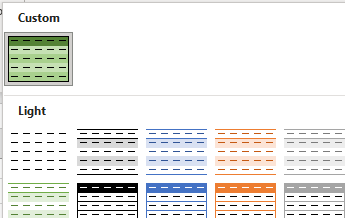
Table Style Options

You can also use table style options to change the appearance of your table.

In the Ribbon, go to Table Design > Table Style Options.

 

 

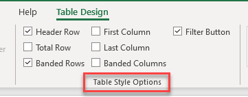
All the options available are toggle checkboxes – you tick them on or off:

• Tick to add or remove the Header Row.
• Tick to show or remove the Total Row.
• To remove alternating row colors, untick Banded Rows.
• To format (or highlight) the first column, tick First Column. You can also do this for the Last Column.
• To add alternating column colors, tick Banded Columns.
• Tick to switch the Filter Buttons at the top of each column on or off.

Change the Table Style in Google Sheets

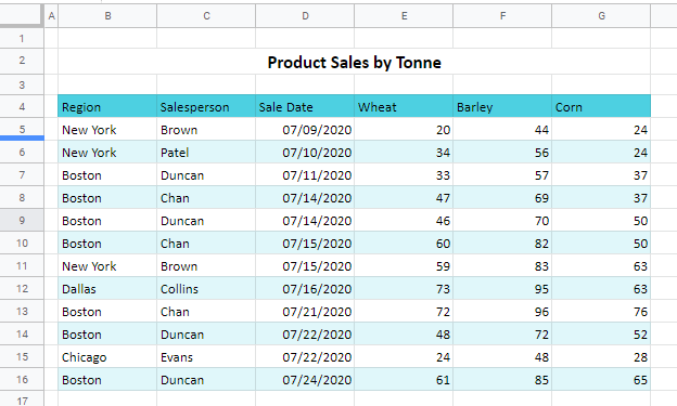
In Google Sheets, you can’t insert a table, but you can format cells with alternating colors.

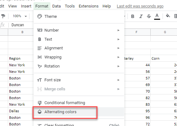
1. Select the data range where you want to display banded rows (B1:E8), and in the Menu, go to Format > Alternating colors.

 

 

2. In the window on the right side, choose a style (e.g., blue). You can also change colors for header and items and make your own custom style. Once you have chosen your colors, click Done.

 

 

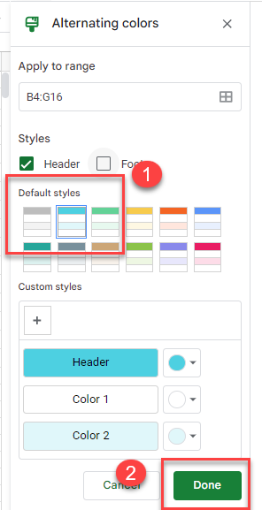
The rows in your range are now banded (alternatively colored).