How to Use Table Tools in Excel

This tutorial demonstrates how to use table tools in Excel.

 

 

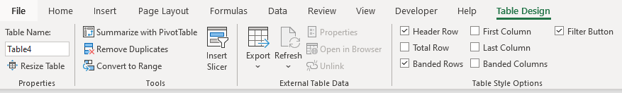
Table Design Tab

The Ribbon in Excel is dynamic. This means that when you insert a table, chart, or pivot table into your worksheet, a new tab appears on your Ribbon which relates to the object you inserted.

1. To get to the Table Design tab, click anywhere within a table and then the tab is visible in the Ribbon, to the right of the Help tab.

 

 

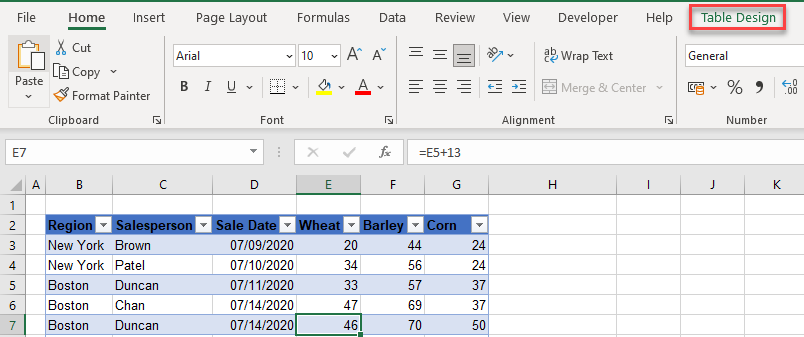
2. Click on this tab in the Ribbon to see the Table Design tab functions.

 

 

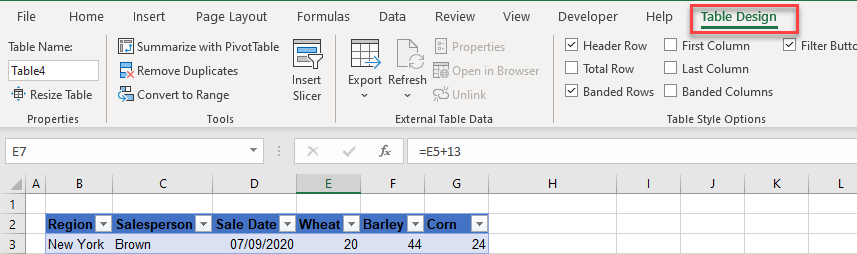
Table Tools

The Tools group offers a few ways to transform or add functionality to an Excel table.

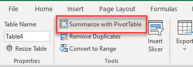
Summarize With Pivot Table

1. In the Tools group of the Ribbon’s Table Design tab, click Summarize with Pivot Table.

 

 

2. The Table/Range box is automatically populated with the table you’re in. Leave the default New Worksheet for where to place the new pivot table, and then click OK.

 

 

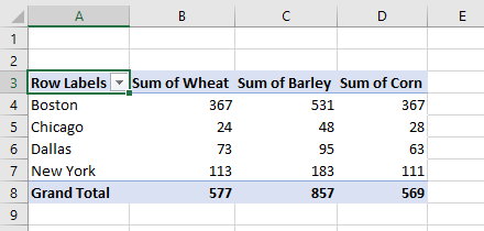
3. A pivot table is placed in a new sheet. Set the Row, Column, and Value fields.

 

 

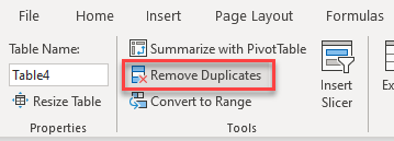
Remove Duplicates

You can remove any repeated information from your table by using the Remove Duplicates tool.

1. In the Tools group of the Table Design tab, click Remove Duplicates.

 

 

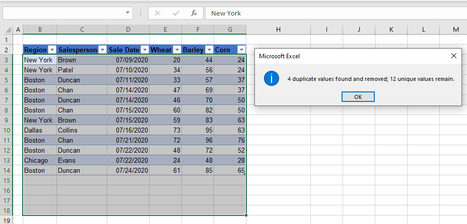
2. In the Remove Duplicates dialog box, tick the columns where there may be duplicates you want to remove. If you only want to remove rows that are identical across all columns, click Select All.

 

 

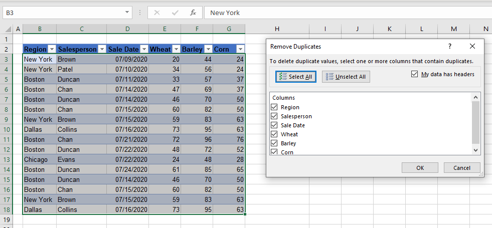
3. Click OK to remove the duplicate rows.

 

 

Convert to Range

If you wish to convert your table to a range (and lose the Table Design tab), You can Convert to Range.

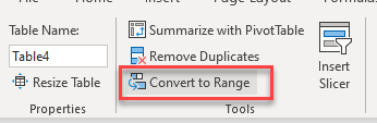
1. In the Tools group of the Table Design tab, click Convert to Range.

 

 

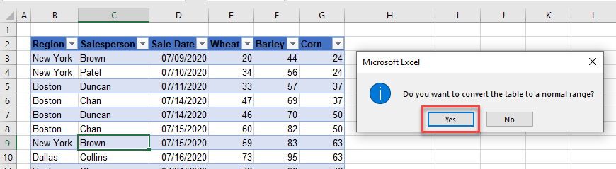
2. Click Yes to convert your table to a range.

 

 

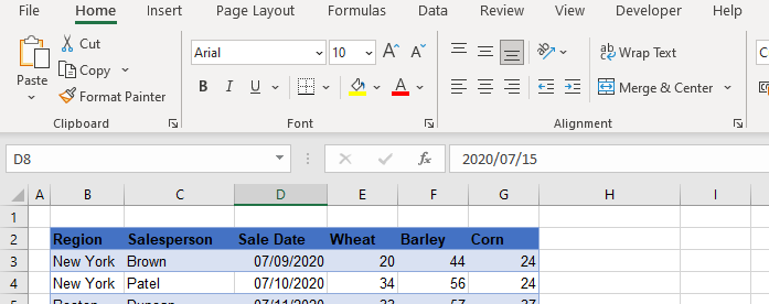
3. Your table is converted to a standard range. Notice that the filter buttons have now been removed and the Table Design tab is no longer available.

 

 

Insert Slicer

As with a pivot table, you are able to create slicers when your data is formatted as a table.

 

 

To filter on more than one option in your slicer, you can hold down the CTRL key (for nonconsecutive values) or the SHIFT key (for consecutive values). Also, try using some shortcuts when you’re working with pivot tables.

Table Styles

You can change the style of your table by using the Table Styles in the Table Design tab on the Ribbon.

 

 

Table Style Options

The Header Row, Total Row, and Filter buttons are all toggle buttons in the Table Style Options group. You can switch these options on or off by clicking in your table, and then ticking the relevant button.

 

 

You can similarly format the first and last columns and to set banded rows and columns in your table.

 

 

Table Properties

The table properties in your Table Design Ribbon allow you to rename and resize a table either by adding rows or columns to the table

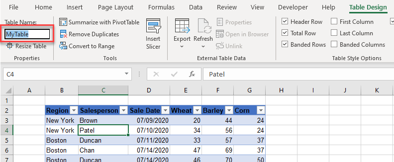
Rename a Table

To rename your table, in the Ribbon, go to Table Design > Properties and then type the name of your table in the name box.

 

 

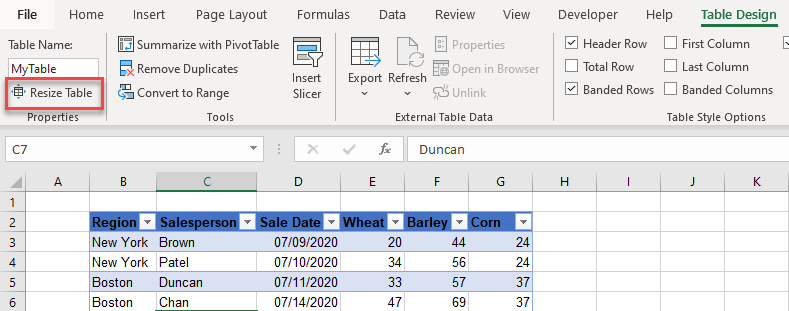
Resize a Table

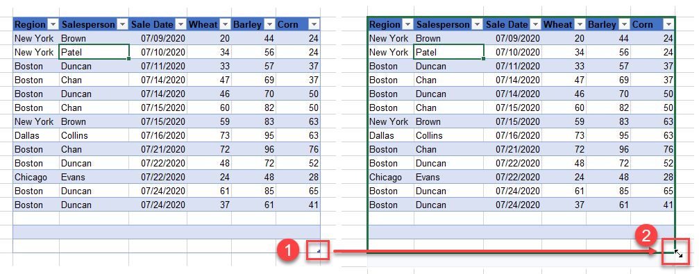
1. To resize your table, in the Ribbon, go to Table Design > Properties > Resize.

 

 

2. Change the range box, either by typing in the new range or by dragging in your worksheet. Click OK.

 

 

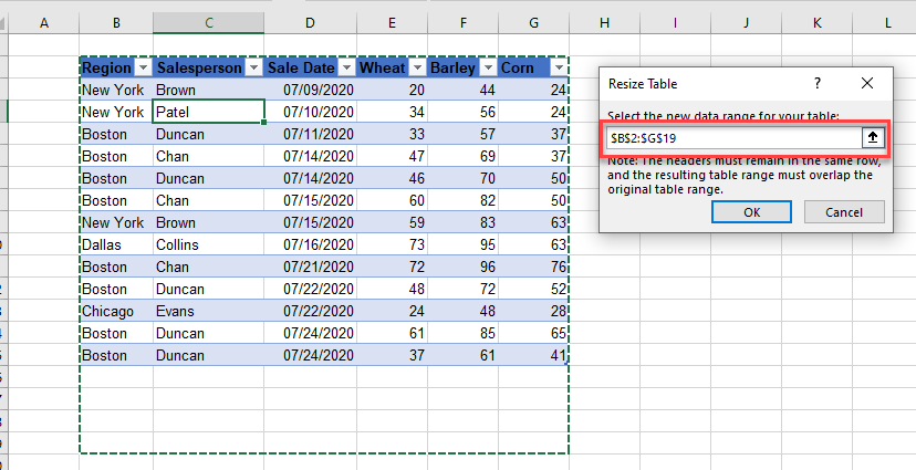
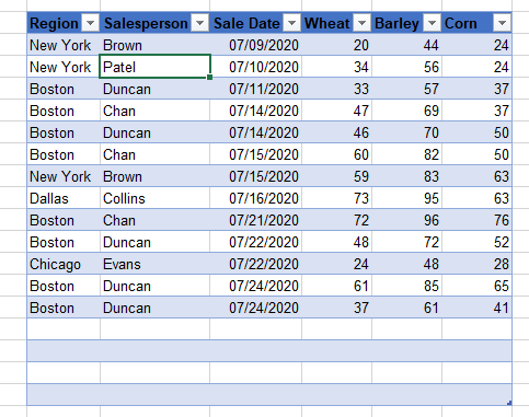
This adjusts the table size based on the selection in the Resize Table dialog box. Compare the pictures above and below.

 

 

3. You can also resize your table by clicking the small handle at the bottom-right corner of the table, and when your mouse turns to a black cross, drag either up or down to add or delete rows, or left or right to add or delete columns.