How to Use Pivot Table Slicers in Excel

This tutorial demonstrates how to use pivot table slicers in Excel.

 

 

One option for manipulating and filtering data in Excel is to use pivot table slicers. Read on for how to create and format slicers, how to use them to filter data, and additional useful settings.

Create Slicer

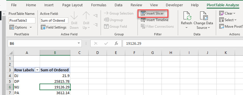
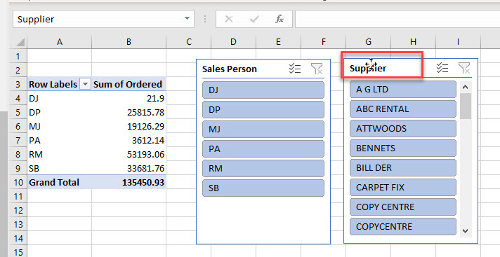
1. Click in your pivot table, and then, in the Ribbon, go to PivotTable Analyze > Insert Slicer.

 

 

2. Tick the slicers to insert.

 

 

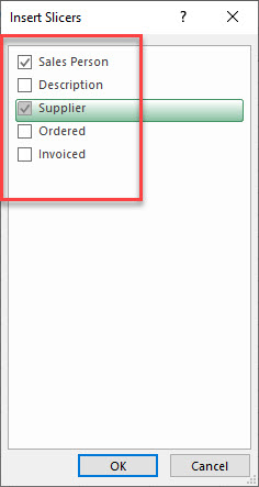
3. Click OK to add these next to your pivot table.

 

 

4. You can drag them around in the current spreadsheet to organize their position on the screen by clicking in the title bar of the slicer and dragging the slicer box across the screen.

 

 

Format Slicer

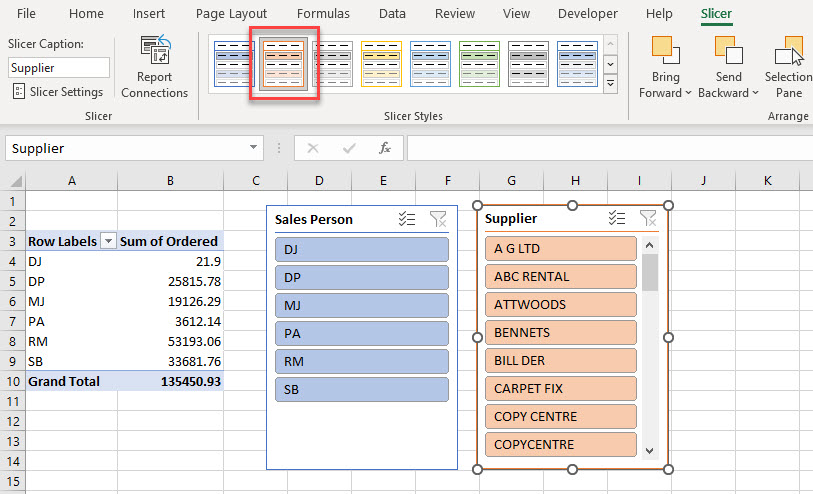
If you want to easily differentiate between the different slicers (if you have added more than one), you can format the slicers to be shown in different colors.

Click on the slicer and a new tab called Slicer is shown in the Ribbon. In this tab, click Slicer Styles, and then choose a style for your slicer.

 

 

Slicers as Filters

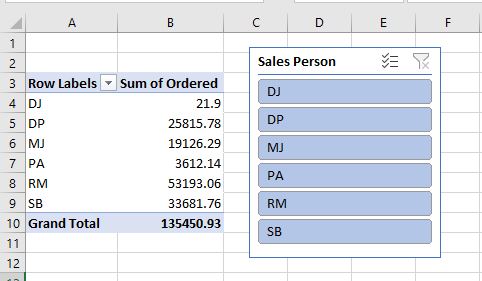
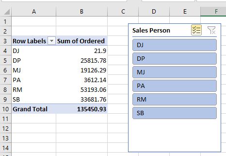
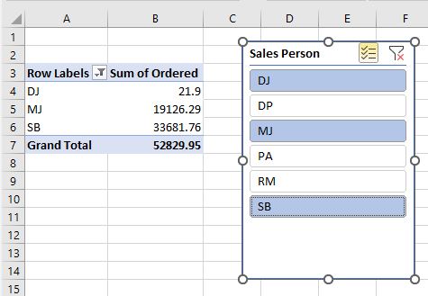
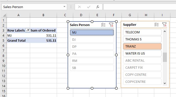
To filter using the slicer, you can add or remove items from the list in the slicer. For example, in the slicer graphic below, all the data is shown by Sales Person.

 

 

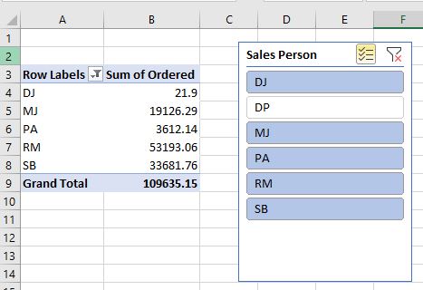
1. Click DP on the slicer to deselect it and filter it out of the data shown in the pivot table. Salesperson DP is excluded.

 

 

2. To only show one salesperson’s data, click each of the other salespeople in the slicer to remove them.

 

 

You can choose more than one entry in the list, so you can filter on more than one salesperson at a time.

 

 

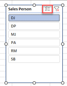
3. To only allow the selection of one item on the list at a time, click to switch off the Multi-Select button (or press ALT + S).

 

 

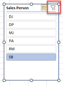
4. To clear the filter and add all the salespeople back into the pivot table, click the Clear Filter button (or press ALT + C).

 

 

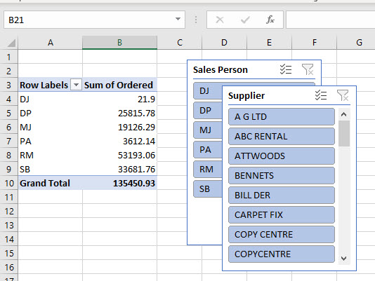
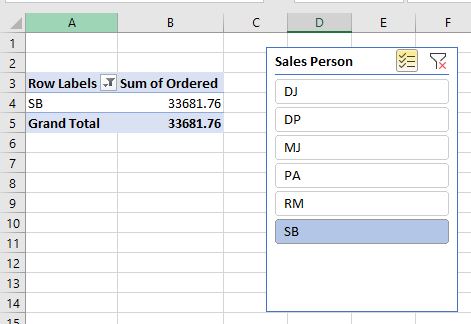
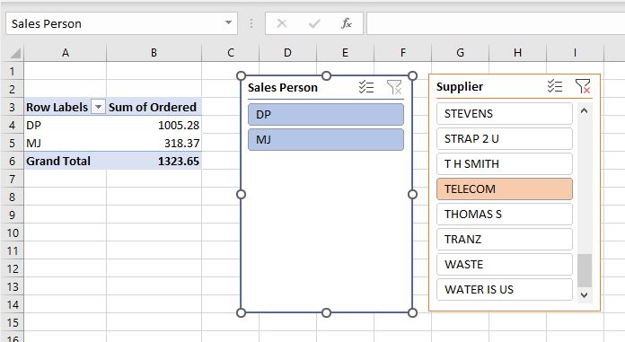
You can now only filter on one item at a time. In the example below, the sum of the Ordered amount is shown for a single salesperson and a single supplier.

 

 

Slicer Settings

There are a few settings you can customize in your slicer, such as sorting the list items into ascending or descending order or hiding items when they don’t exist within the current slicer selection(s).

1. Click on the slicer and then, in the Ribbon, go to Slicers > Slicer Settings.

 

 

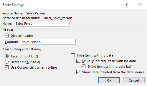
2. Tick Hide items with no data and click OK.

 

 

3. Any items that do not have any data, are removed from the list of items. For example, in the graphic below you are filtering on the supplier Telecom. As there is only data for two salespeople for Telecom, only these two items are shown on the Sales Person slicer.

 

 

Tip: Try using some shortcuts when you’re working with pivot tables.