How to Filter Pivot Table Values in Excel & Google Sheets

This tutorial demonstrates how to filter pivot table values in Excel and Google Sheets.

 

 

Built-in Pivot Table Filter

When you create a pivot table, the column headers from the data become fields for the pivot table. Filtering in a pivot table is similar to applying any other filter in Excel.

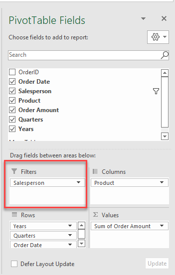
1. In the PivotTable Fields window, drag fields down to one of four areas to build the table. One area is for Filters.

 

 

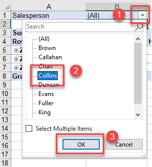
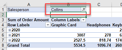
2. You can then filter your pivot table by the field(s) from the Filters area (here, Salesperson). Find the filter field(s) at the top of your pivot table, above column headings and a blank row. Click the arrow for the filter field and choose the item to filter on (e.g., Collins). Then click OK.

 

 

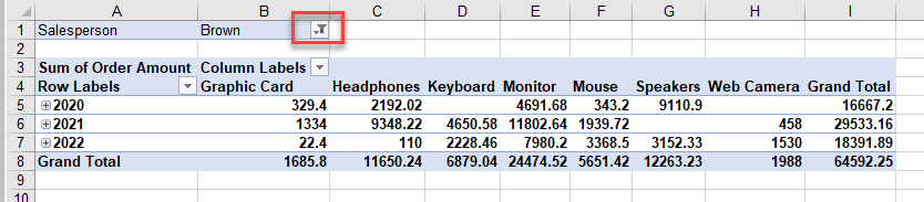
Now the pivot table shows all the information set up in the PivotTable Fields window, but only for rows where the Salesperson is Collins.

 

 

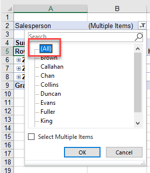
3. To clear the filter, click the filter drop down on the right side of the cell. Choose (All) then click OK.

 

 

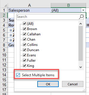
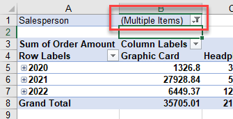
4. If you want to filter on multiple items, tick Select Multiple Items. Notice how each item in the drop down now has a checkbox next to it.

 

 

5. Uncheck the (All) box and tick the items you wish to filter on (e.g., Chan and Collins). Click OK.

 

 

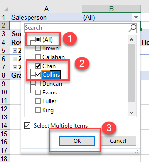
The cell with the filter drop down (here, B1) shows that multiple items are included, but you cannot see which items without clicking the arrow on the right.

 

 

6. To clear the filter once again, choose (All) from the filter drop down and click OK.

Filter by Row / Column

You can also filter by the row and column labels.

1. Click the filter drop down to the right of the Column Labels heading. Remove the checkmark from (Select All), and then tick the item you wish to filter on.

 

 

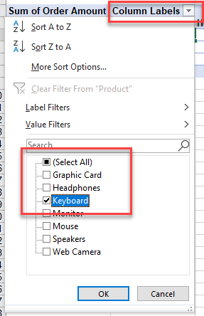
2. Click OK to apply the filter.

 

 

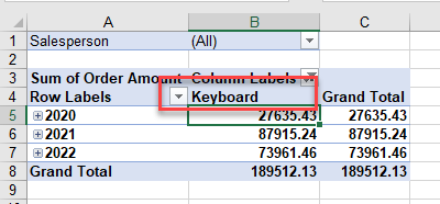
Filter Row Labels in the same way.

 

 

Filter Values by Date

If you have dates in your pivot table, you can filter by these dates. This can be done in the Filters, Rows, and/or Columns areas.

Filter by Year or Quarter

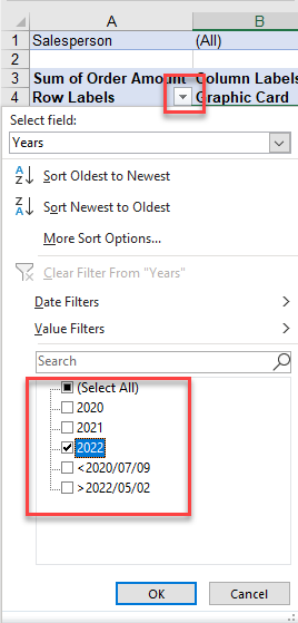
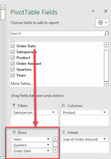
When a date is added to the Rows or Columns area, it is automatically broken down into three groups – Years, Quarters, and the actual value of the date field itself. All three fields are added to the relevant area.

 

 

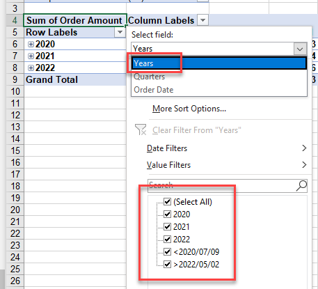
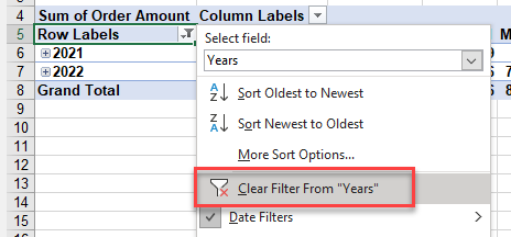
You can then click the Row Labels filter drop down and choose the specific field to filter on (e.g., Years) in the Select field drop down.

 

 

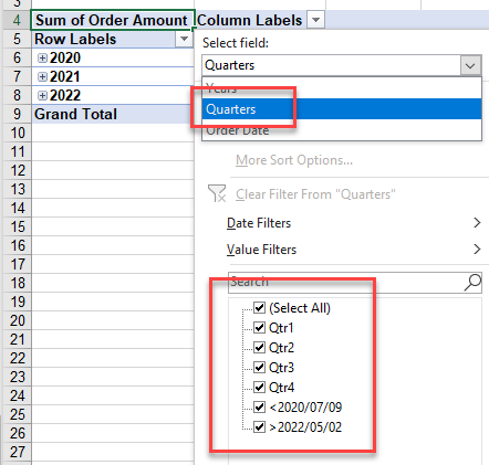
Also try changing the filter field to filter by quarters instead of years.

 

 

Filter by Month

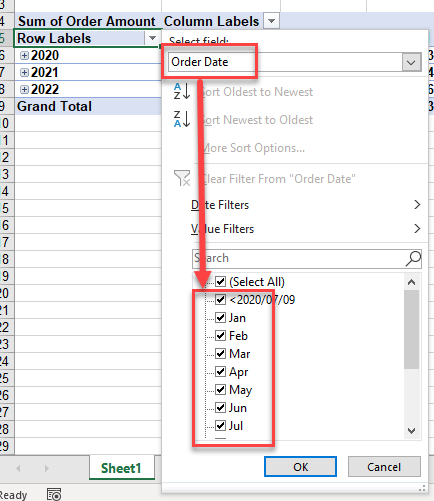
To filter by month, choose the original field (e.g., Order Date) from the drop down instead of the automatically generated years or quarters.

 

 

Other Date Filters

You can also choose Date Filters from the Row Labels drop down, and then choose the criteria you need – for example, This Year.

 

 

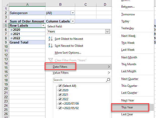
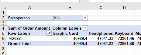
This immediately restricts the data shown to this year only.

 

 

Date Range

You can also be more specific and choose the start and end dates to filter on.

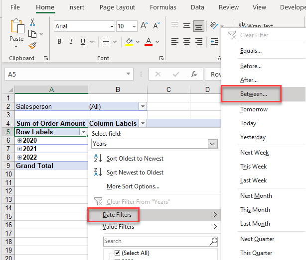
1. From the Row Labels drop down, go to Date Filters > Between…

 

 

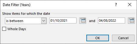
2. Select the start and end dates and click OK.

 

 

Notice a small icon in the Row Labels drop down (on the right side of the cell) indicating that a filter is applied.

 

 

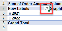
3. To get rid of the filter, click Clear Filter from “Years” in the drop down.

 

 

Add Additional Filters

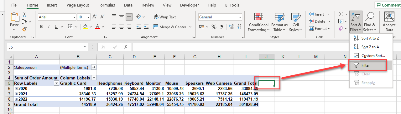
Individual columns of a pivot table do not have filters automatically in place.

1. To create a filter on these values, select the cell to the right of the pivot table (here, J5), and then in the Ribbon, go to Home > Editing > Filter.

 

 

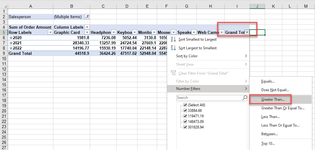
2. This adds a filter to each column label. You can then filter on each value. For example, you can tick any of the individual values in the Grand Total list, or you can use a Number Filter, such as one that includes only values Greater Than a certain amount.

 

 

Tip: Try using some shortcuts when you’re working with pivot tables.

Filter Pivot Table in Google Sheets

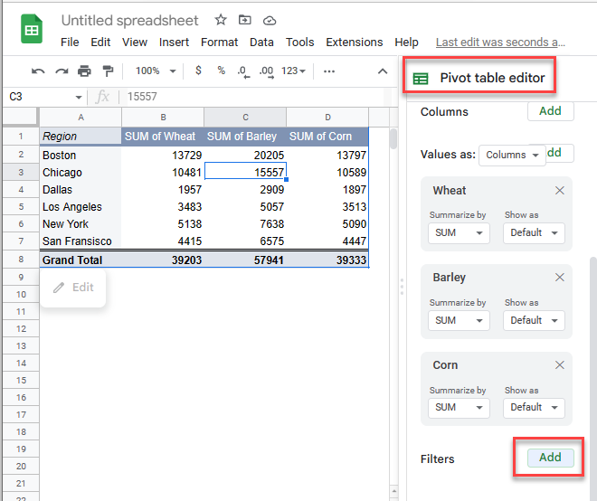
Pivot tables, especially the window where the table is built and structured, look a little different in Google Sheets, but the methods for filtering are similar.

1. In the Pivot table editor, click Add.

 

 

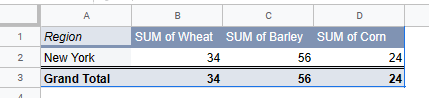
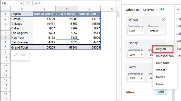
2. Choose the field you wish to filter on (e.g., Region).

 

 

3. Under Filter by values, click Clear. Then individually tick the values to include in the filter.

 

 

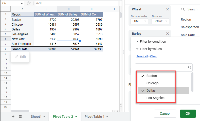
4. Click OK to apply the filter.

 

 

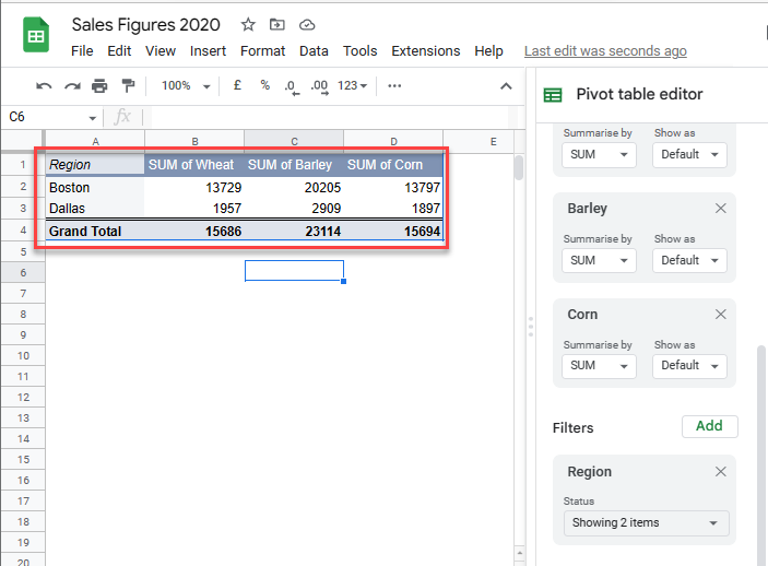
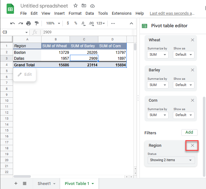
5. To clear the filter, click the X to the right of the filtered field.

 

 

Filter by Condition

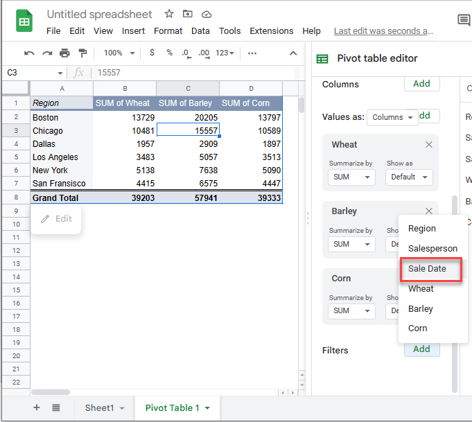
1. Now, add a filter for the Sale Date to the pivot table.

 

 

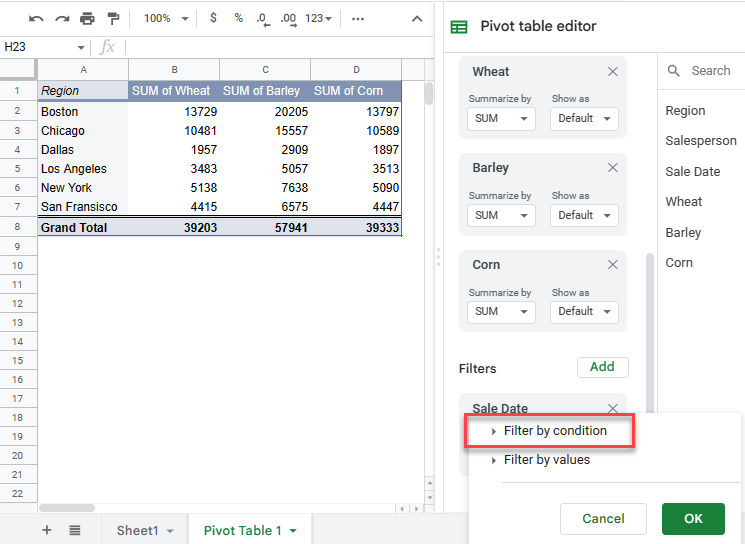
2. Click Filter by condition.

 

 

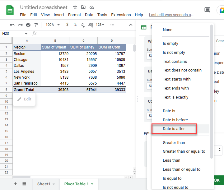
3. Choose Date is after from the drop down.

 

 

4. Then, click exact date from the next drop down.

 

 

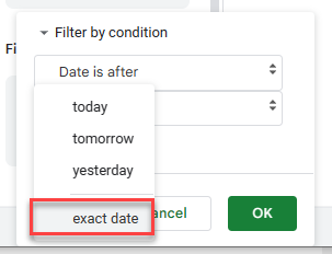
5. In the bottom box, type in the date you need. Click OK.

 

 

The pivot table is filtered accordingly.