Compare Two Columns for Matches in Excel & Google Sheets
Written by
Reviewed by
This tutorial demonstrates how to compare two columns for matches in Excel and Google Sheets.
Compare Columns Side by Side
If you have data in two columns that may or may not be adjacent to each other, you can use a formula in a third column to check to see if the data in the first and second columns match.

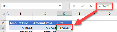
- To check if the figure in B3 matches the figure in C3, enter the following formula:
=B3=C3If the figures match, a TRUE is returned; otherwise a FALSE is returned.
- Copy the formula down to the end of the data to see which figures match in the columns.
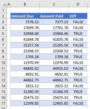
- Go down Column D and use TRUE results to identify matching rows.
One benefit of this method is that TRUE and FALSE are values in Excel, so Column D can be used in formulas if needed.
See also…
- How to View Two Sheets From the Same Workbook
- How to Compare Two Sheets for Differences
- How to Compare Two Files for Differences
Compare Using Conditional Formatting
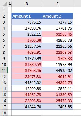
You can also highlight matching values using conditional formatting.
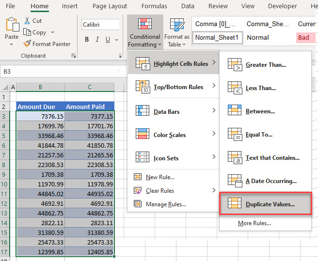
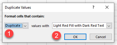
- Select data in the columns you want to compare and in the Ribbon, go to Home > Conditional Formatting > Highlight Cells Rules > Duplicate Values.
- In the pop-up window, leave Duplicate selected, and click OK. You can leave the default format (Light Red Fill with Dark Red Text).
- Visually identify matching values in the lists based on which rows are highlighted.
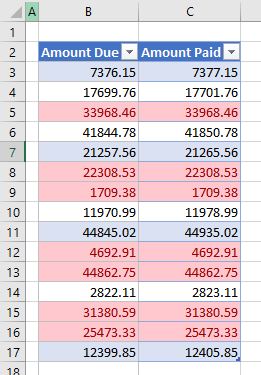
This method can be used to see if there are duplicate numbers between two columns even if the numbers are not in the same row.
See also…
Compare With VLOOKUP
A third way of seeing if the data in Column 1 matches the data in Column 2 is to use the VLOOKUP Function.
- Enter:
=VLOOKUP(C3,$B$3:$B$17,1,FALSE)
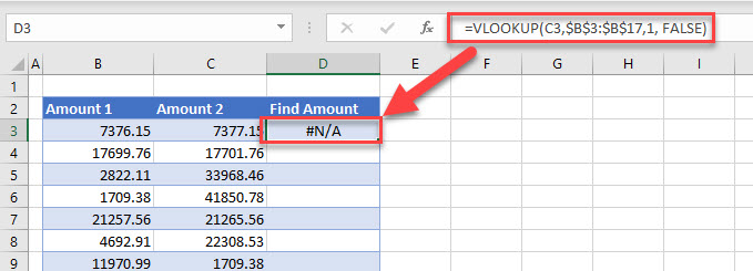
The formula above returns #N/A as it does not find the value that is held in C3 in any of the cells in the Range B3:B17.
- Copy this formula down to Row 17 to find matching values.
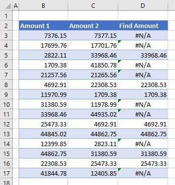
- Where there is a matching value, the value will show in Column D. Otherwise, a #N/A error will appear.
See also…
- VLOOKUP Contains (Partial Match)
- VLOOKUP – Display Multiple Matches (Rows of Results)
- VLOOKUP – Multiple Results with VBA
Compare Two Columns for Matches in Google Sheets
In Google Sheets, you can compare two columns side by side and by using the VLOOKUP Function in the same way as you do in Excel.
For Conditional Formatting, however, the process is slightly different.
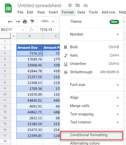
- Select one of the ranges you want to compare (B2:C9), and in the Menu, go to Format > Conditional formatting.
- In the window on the right side, (1) select Custom formula is under Format rules and (2) enter the formula:
=$B2=$C2Then (3) click on the fill color icon, (4) choose orange, and (5) click Done.
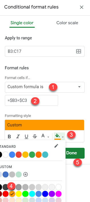
The formula has a dollar sign to fix columns, only changing rows. This means that the formatting rule will go row by row and compare cells in Columns B and C.
- Visually identify matching values in the columns: Cells with the same values have an orange fill color.

