VLOOKUP Contains (Partial Match) – Excel & Google Sheets
Written by
Reviewed by
Download the example workbook
This tutorial will demonstrate how to perform a partial match VLOOKUP in Excel.
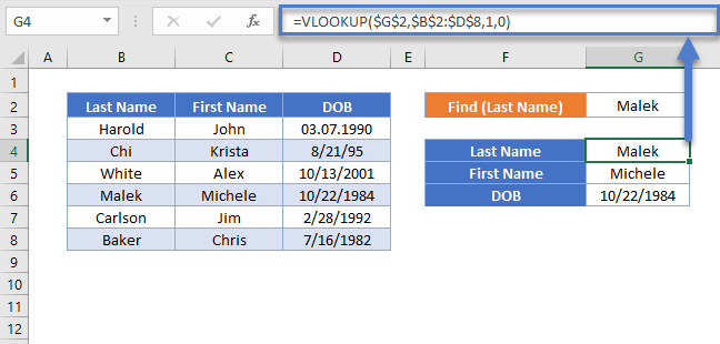
VLOOKUP Function
The VLOOKUP Function lookups a value in the leftmost column of a range and returns a corresponding value from another column.
Partial Match VLOOKUP (Text Contains)
By using the asterisk “wildcard” (*), within a VLOOKUP, we can lookup values that contain (partial match) certain text, instead of values that match the lookup text exactly. Let’s walk through an example.
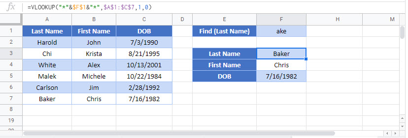
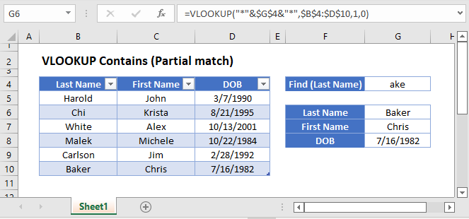
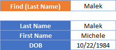
Here we have a list of names and want to find a name that contains “ake”.
To accomplish this, we combine VLOOKUP with a wildcard in a formula like so:
=VLOOKUP("*"&<Partial Value>&"*",<lookup range>,<match column position>,0)=VLOOKUP("*"&$G$2&"*",$B$2:$D$8,1,0)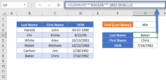
The formula merges “ake” with the “*” wildcards, using the “&” symbol. Because the “*” wildcard is before and after the lookup text, the VLOOKUP Function will look for “ake” anywhere in the lookup range. Instead you could add “*” only before the text to lookup values that end in the lookup text. Or “*” after the lookup value for values that begin with the lookup text.
Limitation: wildcards only work with VLOOKUP function in exact mode (0 or FALSE for the [range lookup] parameter)
VLOOKUP Contains (Partial Match) in Google Sheets
These formulas work exactly the same in Google Sheets as in Excel.