VLOOKUP Function Examples – Excel & Google Sheets
Written by
Reviewed by
Download the example workbook
This Tutorial demonstrates how to use the Excel VLOOKUP Function in Excel to look up a value.
VLOOKUP Function Overview
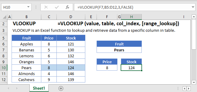
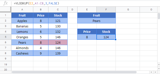
The VLOOKUP Function Vlookup stands for vertical lookup. It searches for a value in the leftmost column of a table. Then returns a value a specified number of columns to the right from the found value. It is the same as a hlookup, except it looks up values vertically instead of horizontally.
![]()
(Notice how the formula inputs appear)
VLOOKUP Function Syntax and Arguments:
=VLOOKUP(lookup_value,table_array,col_index_num,range_lookup)lookup_value – The value you want to search for.
table_array – The data range that contains both the value you want to search for and the value you want the vlookup to return. The column containing the search values must be the left-most column.
col_index_num – The column number of the data range, from which you want to return a value from.
range_lookup – TRUE or FALSE. FALSE searches for an exact match. TRUE searches for the nearest match that is less than or equal to the lookup_value. If TRUE is chosen the left-most column (the lookup column) must be sorted ascendingly (lowest to highest).
What is the VLOOKUP function?
As one of the older functions in the world of spreadsheets, the VLOOKUP function is used to do Vertical Lookups. It has a few limitations that are often overcome with other functions, such as INDEX/MATCH. However, it does have the benefit of being a single function that can do an exact match lookup by itself. It also tends to be one of the first functions people learn about.
Basic example
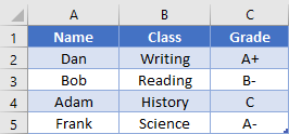
Let’s look at a sample of data from a grade book. We’ll tackle several examples for extracting information for specific students.
If we want to find what class Bob is in, we would write the formula:
=VLOOKUP("Bob", A2:C5, 2, FALSE)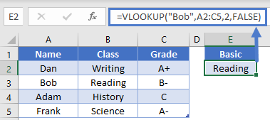 Important things to remember are that the item we’re searching for (Bob), must be in the first column of our search range (A2:C5). We’ve told the function that we want to return a value from the 2nd column, which in this case is column B. Finally, we indicated that we want to do an exact match by placing False as the last argument. Here, the answer will be “Reading”.
Side tip: You can also use the number 0 instead of False as the final argument, as they have the same value. Some people prefer this as it’s quicker to write. Just know that both are acceptable.
Shifted Data
To add some clarification to our first example, the lookup item doesn’t have to be in column A of your spreadsheet, just the first column of your search range. Let’s use the same data set:
Now, let’s find the grade for the class of Science. Our formula would be
=VLOOKUP("Science", B2:C5, 2, FALSE)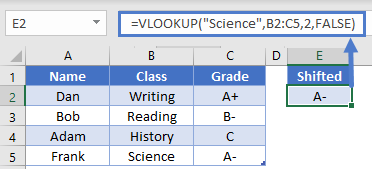 This is still a valid formula, as the first column of our search range is column B, which is where our search term of “Science” will be found. We’re returning a value from the 2nd column of the search range, which in this case is column C. The answer then is “A-“.
Wildcard usage
The VLOOKUP function supports the use of the wildcards “*” an “?” when doing searches. For instance, let’s say that we’d forgotten how to spell Frank’s name, and just wanted to search for a name that starts with “F”. We could write the formula
=VLOOKUP("F*", A2:C5, 2, FALSE)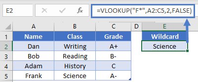
This would be able to find the name Frank in row 5, and then return the value from 2nd relative column. In this case, the answer will be “Science”.
Non-exact match
Most of the time, you’ll want to make sure that the last argument in VLOOKUP is False (or 0) so that you get an exact match. However, there are a few times when you might be searching for a non-exact match. If you have a list of sorted data, you can also use VLOOKUP to return the result for the item that is either the same, or next smallest. This is often used when dealing with increasing ranges of numbers, such as in a tax table or commission bonuses.
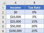
Let’s say that you want to find the tax rate for an income entered cell D2. The formula in D4 can be:
=VLOOKUP(D2, A2:B6, 2, TRUE)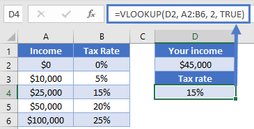
The difference in this formula is that our last argument is “True”. In our specific example, we can see that when our individual inputs an income of $45,000 they will have a tax rate of 15%.
Note: Although we usually are wanting an exact match with False as the argument, it you forget to specify the 4th argument in a VLOOKUP, the default is True. This can cause you to get some unexpected results, especially when dealing with text values.
Dynamic column
VLOOKUP requires you to give an argument saying which column you want to return a value from, but the occasion may arise when you don’t know where the column will be, or you want to allow your user to change which column to return from. In these cases, it can be helpful to use the MATCH function to determine the column number.
Let’s consider our grade book example again, with some inputs in E2 and E4. To get the column number, we could write a formula of
=MATCH(E2, A1:C1, 0)This will try to find the exact position of “Grade” within the range A1:C1. The answer will be 3. Knowing this, we can plug it into a VLOOKUP function and write a formula in E6 like so:
=VLOOKUP(E4, A2:C5, MATCH(E2, A1:C1, 0), 0)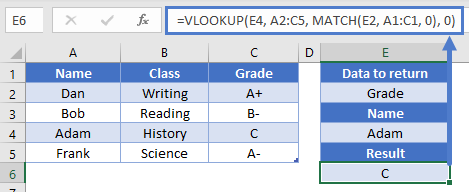
So, the MATCH function will evaluate to 3, and that tells the VLOOKUP to return a result from the 3rd column in the A2:C5 range. Overall, we then get our desired result of “C”. Our formula is dynamic now in that we can change either the column to look at or the name to search for.
VLOOKUP limitations
As mentioned at the beginning of the article, the biggest downfall of VLOOKUP is that it requires the search term to be found in the left most column of the search range. While there are some fancy tricks you can do to overcome this <link to CHOOSE article>, the common alternative is to use INDEX and MATCH. That combo gives you more flexibility, and it can sometimes even be a faster calculation.
VLOOKUP in Google Sheets
The VLOOKUP Function works exactly the same in Google Sheets as in Excel:
Additional Notes
Use the VLOOKUP Function to perform a VERTICAL lookup. The VLOOKUP searches for an exact match (range_lookup = FALSE) or the closest match that is equal to or less than the lookup_value (range_lookup = TRUE, numeric values only) in the first row of the table_array. It then returns a corresponding value, n number of rows below the match.
When using an VLOOKUP to find an exact match, first you define an identifying value that you want to search for as the lookup_value. This identifying value might be a SSN, employee ID, name, or some other unique identifier.
Next you define the range (called the table_array) that contains the identifiers in the top row and whatever values that you ultimately wish to search for in the rows below it. IMPORTANT: The unique identifiers must be in the top row. If they are not, you must either move the row to the top, or use MATCH / INDEX instead of the VLOOKUP.
Third, define row number (row_index) of the table_array that you wish to return. Keep in mind that the first row, containing the unique identifiers is row 1. The second row is row 2, etc.
Last, you must indicate whether to search for an exact match (FALSE) or nearest match (TRUE) in the range_lookup. If the exact match option is selected, and an exact match is not found, an error is returned (#N/A). To have the formula return blank or “not found”, or any other value instead of the error value (#N/A) use the IFERROR Function with the VLOOKUP.
To use the VLOOKUP Function to return an approximate match set: range_lookup = TRUE. This option is only available for numeric values. The values must be sorted in ascending order.
To perform a horizontal lookup use the HLOOKUP Function instead.
VLOOKUP Examples in VBA
You can also use the VLOOKUP function in VBA. Type:
application.worksheetfunction.vlookup(lookup_value,table_array,col_index_num,range_lookup)For the function arguments (lookup_value, etc.), you can either enter them directly into the function, or define variables to use instead.
Return to the List of all Functions in Excel

