Compare Two Sheets for Differences in Excel & Google Sheets

This tutorial demonstrates how to compare two sheets for differences in Excel and Google Sheets.

Compare Sheets Side by Side

You can compare two sheets in Excel side by side by opening a new window in the active file using the New Window button on the View menu. You can also use this feature to view two files at the same time.

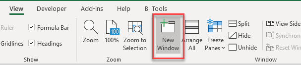
1. Make sure you have a file open that contains multiple worksheets and then, in the Ribbon, go to View > New Window.

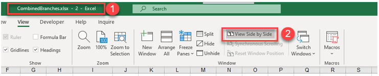
2. You can switch to the new window and move to a different sheet. The (1) title bar in Excel will show that you have two windows of the same book by adding a 2 after the file name. To view the sheets side by side, click (2) View Side by Side.

The default setting for View Side by Side is for one of the windows to be

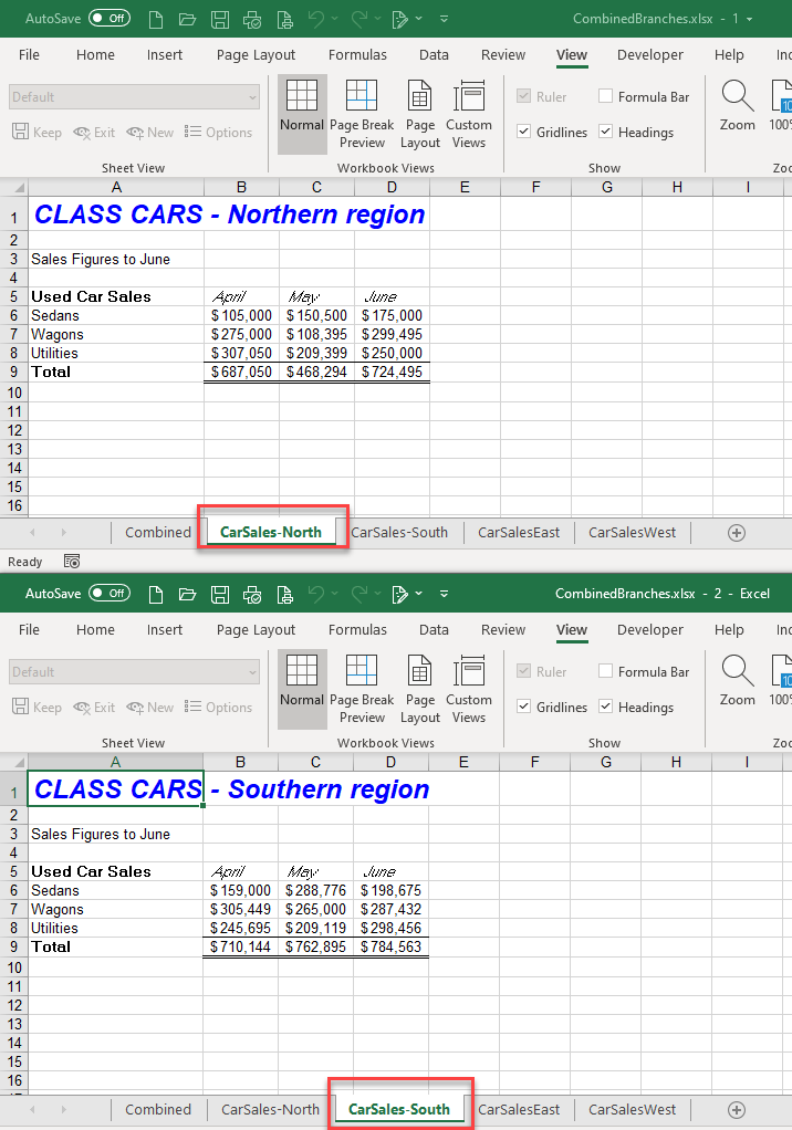
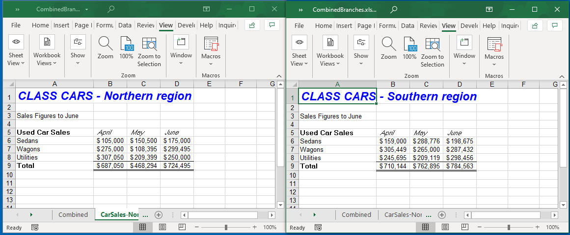
3. To view the sheets next to each other instead of one below the other, in the Ribbon, go to View > Arrange All, choose Vertical, and then click OK.

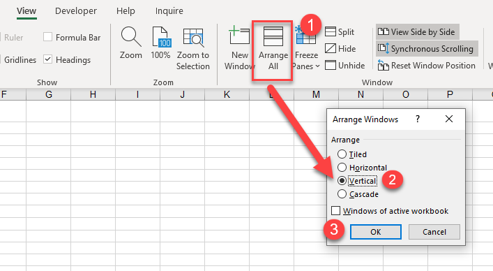
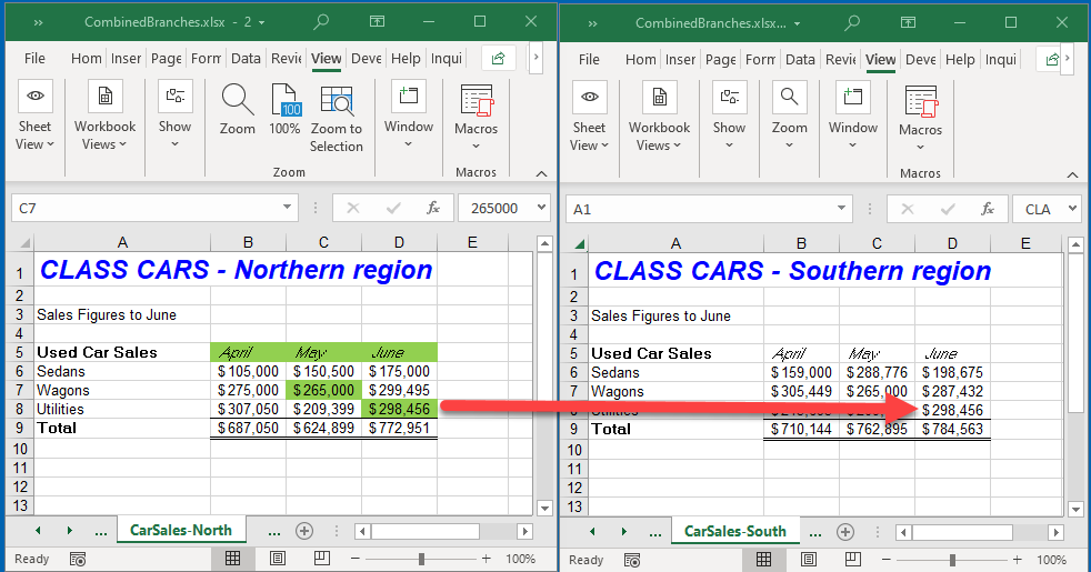
The two windows are displayed next to each other on your screen.

4. You can now visually compare the data in the two sheets to see the differences. You can also use this method to compare two separate files for differences.

Compare Using Conditional Formatting

You can compare the values in the same cells in two separate sheets with conditional formatting.

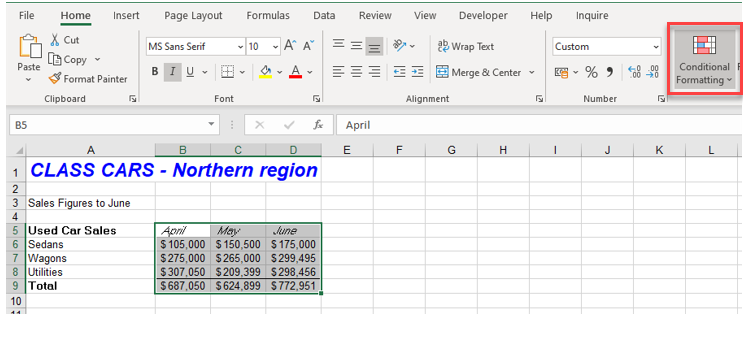
1. Highlight the cells in the first sheet that you wish to compare and then, in the Ribbon, go to Home > Conditional Formatting.

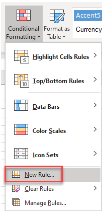
2. In the Conditional Formatting menu, choose New Rule.

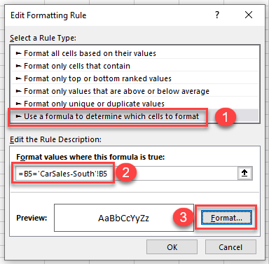
3. Choose Use a formula to determine which cells to format. Then type in the formula:

   =B5='CarSales-South'!B5

   where CarSales-South is the name of the sheet you’re comparing to the active sheet.
   Note: Do not use $ signs (absolutes) around the cell addresses!
   Finally, click Format.

4. Go to the Fill tab, and then choose the color to apply to cells meeting the conditional formatting criteria. Click OK.

5. Click OK until you’re back to the Excel sheet. Any cells that are equal to each other in the two sheets being compared are highlighted in green.

Compare With Formulas

You can get even more detailed in comparing the two sheets by creating a third sheet to use as a “report” sheet.

1. In the Excel file where the report is required, add a new sheet (in this example, called ComparisonReport).

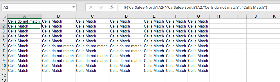
2. In Cell A1 of the new sheet, type the following IF formula:

   =IF('CarSales-North'!A1<>'CarSales-South'!A1,"Cells do not match", "Cells Match")

   where CarSales-North and CarSales-South are the names of the two sheets whose data you are comparing.

3. Copy this formula down and across to the amount or rows and columns that are populated in the original sheets.

Compare Sheets for Differences in Google Sheets

To compare two sheets for differences in Google Sheets, you can use the formula approach as described above.

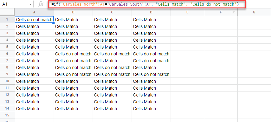
In your Google file, create a new sheet called ComparisonReport and then type the formula in cell A1 to compare the relevant sheets:

=IF('CarSales-North'!A1='CarSales-South'!A1,"Cells Match", "Cells do not match")