Compare Two Columns and Highlight Differences in Excel & Google Sheets
Written by
Reviewed by
This tutorial demonstrates how to compare two columns and highlight differences in Excel and Google Sheets.
Shortcut to Select Differences
Read on for how to apply formatting to the differences.
Compare Two Columns and Highlight the Differences
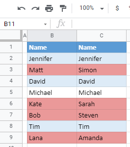
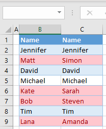
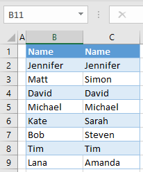
In Excel, you can compare two columns and highlight their differences using conditional formatting. Say you have the following data with two lists of names in Columns B and C.
To highlight all differences (Rows 3, 6, 7, and 9) in red, follow these steps:
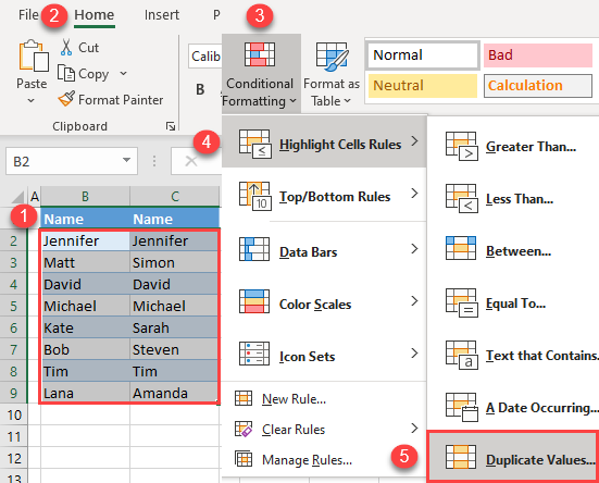
- Select data in the columns you want to compare and in the Ribbon, go to Home > Conditional Formatting > Highlight Cells Rules > Duplicate Values.
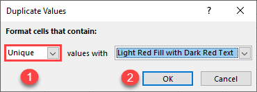
- In the pop-up window, (1) select Unique and (2) click OK. You can leave the default format (Light Red Fill with Dark Red Text).
You could also have selected Duplicate; in that case, the same values would be highlighted.
As a result, cells containing different values in Columns B and C are highlighted in red.
Compare Two Columns in Google Sheets
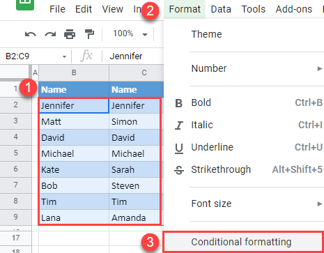
You can also compare two columns using conditional formatting in Google Sheets.
- Select a data range you want to compare (B2:C9), and in the Menu, go to Format > Conditional formatting.
- In the window on the right side, (1) select Custom formula is under Format rules and (2) enter the formula:
=$B2<>$C2Then (3) click on the fill color icon, (4) choose red, and (5) click Done.
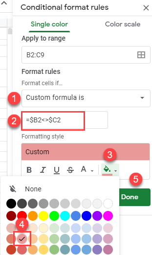
The formula has a dollar sign to fix columns, only changing rows. This means that the formatting rule will go row-by-row and compare cells in Columns B and C.
As a result, cells with different values have a red fill color.