Conditional Formatting Based on Formula – Excel & Google Sheets

This tutorial demonstrates how to apply conditional formatting based on a formula in Excel and Google Sheets.

 

 

Conditional Formatting in Excel comes with plenty of preset rules to enable you to quickly format cells according to their content. These preset rules do, however, have limitations, which is where using a formula to determine the format of a cell comes into play. This gives you much greater flexibility over your conditional formatting.

Conditional Formatting Formula Rules

Equal To

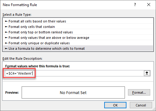
1. Highlight the cells where you want to set the conditional formatting and then, in the Ribbon, select Home > Conditional Formatting > New Rule.

 

 

2. Select Use a formula to determine which cells to format, and enter the formula:
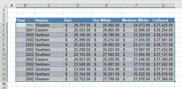
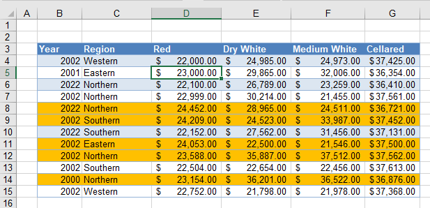
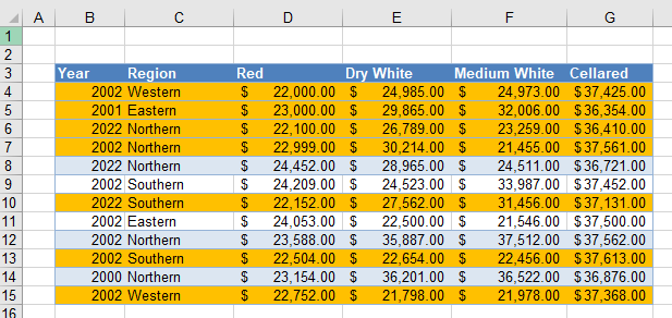
   =$C4=”Western”

 

 

You always need to start your formula with an equal sign.

The formula tests whether the result is TRUE or FALSE much like the traditional Excel IF statement, but in the case of conditional formatting, you do not need to add the true and false conditions. If the formula returns TRUE, then formatting you set in the Format part of the rule is applied to the relevant cells.

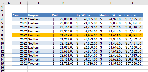
You need to use a mixed reference in this formula ($C4) in order to lock the column (make it absolute) but make the row relative. This enables the formatting to format the entire row instead of just a single cell that meets the criteria.

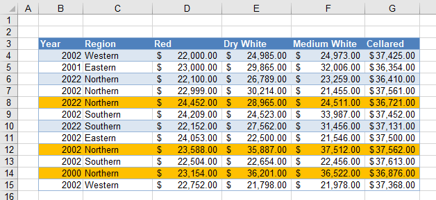
When the rule is evaluated for all the cells in the range, the row changes, but the column does not. This causes the rule to ignore the values in any of the other columns and just concentrate on the values in Column C. If Column C of that row contains the word Western, the formula result is TRUE, and the formatting is applied for the whole row.

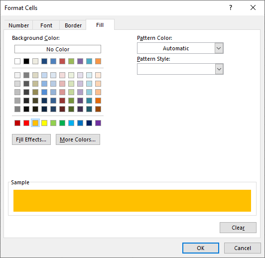
3. Click Format… and select your desired formatting.

 

 

4. Click OK and then OK again to view the result.

 

 

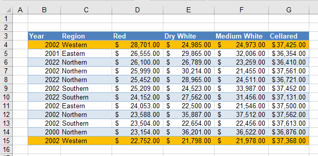
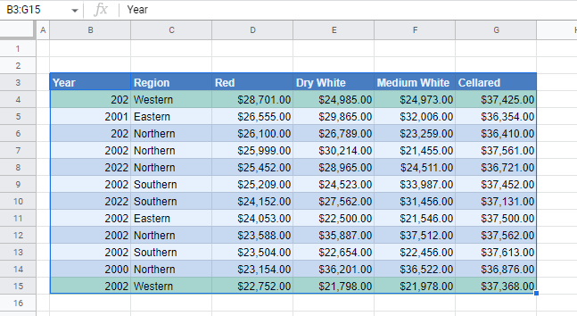
The rows where Column C is Western are highlighted, while other rows are not. In the example above, just two rows end up highlighted.

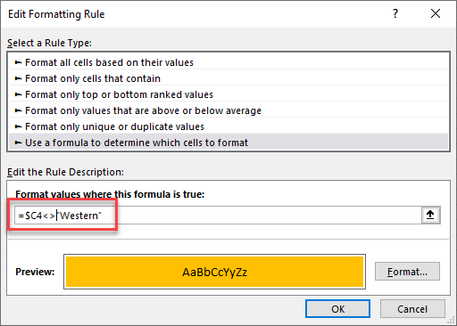
Not Equal

If you want to create an opposite rule, you can use the <> (not equal to) operator instead of =.

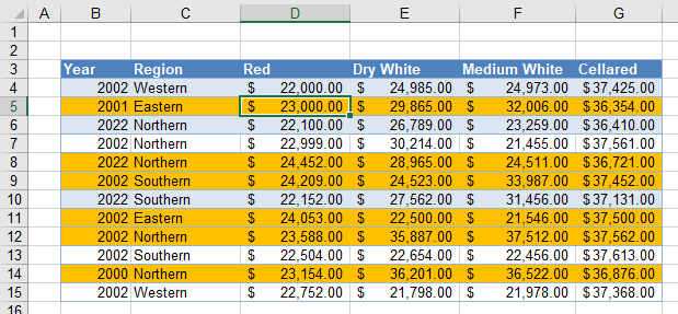
=$C4<>”Western”

 

 

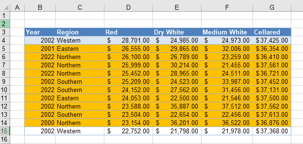
This results in the opposite: Most of the rows are now highlighted!

 

 

Greater Than

You can also test for greater than using a formula. For example, you can use a formula to check if the values in Column D are greater than $23,000.

=$D4>23000

 

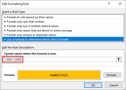
This rule highlights only rows where the value in Column D is greater than $23,000.

 

 

Greater Than or Equal To

Similarly, you could highlight the rows where the value in Column D is greater than or equal to $23,000 with this formula below:

=$D4>=23000

 

 

The result for this formula would be slightly different: Rows where the Red value is exactly $23,000 are also highlighted (here, Row 5).

 

 

Less Than

Swapping the > sign for a < sign tests for values that are less than $23,000.

=$D4<23000

 

 

Now only rows where Red is less than $23,000 are highlighted.

 

 

Less Than or Equal To

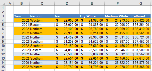
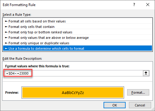
To change the test to include the target value (e.g., $23,000), use <=.

=$D4<=23000

 

 

Now, any rows in which Column D is equal to $23,000 are also highlighted.

 

 

Create Rules With OR, AND

OR Formula

You can create a more complicated rule by incorporating the Excel OR Function to expand the formula to look for two or more values.

1. Enter the formula:
   =OR($C4=”Western”,$C4=”Eastern”)

 

 

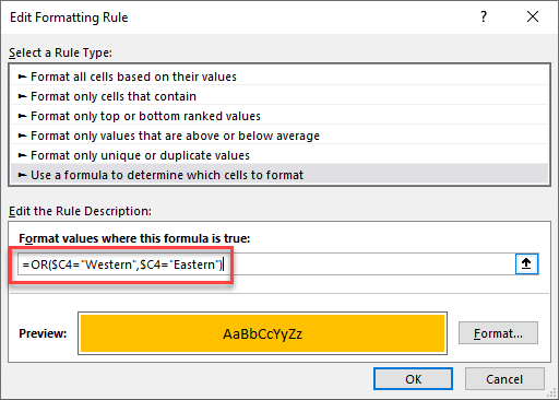
2. Click on the Format… button and select your desired formatting, and then click OK to return to Excel.

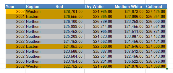
This highlights all rows where the Region is Western or Eastern.

 

 

AND Formula

Similarly, you can create a rule using AND. This would mean checking the values in two or more columns.

 

 

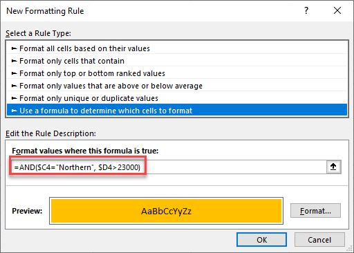
The formula above checks whether the text in Column C is Northern and the value in the corresponding row in Column D is greater than $23,000.

 

 

This conditional formatting rule highlights only the rows where both conditions are met.

IF Formula

You do not necessarily have to add an IF statement to the formula when you are creating it in a conditional formatting rule as the conditional formatting is always going to apply the rule if the formula that you have created returns a true value.

So, for example, this formula:

=IF($C4=”Western”,TRUE,FALSE)

and this formula

$C4=”Western”

both apply the same conditional formatting to your worksheet.

Built-in Excel Functions

Many built-in Excel functions can be used in conditional formatting such as ISBLANK, ISERROR, ISEVEN, ISNUMBER, etc.

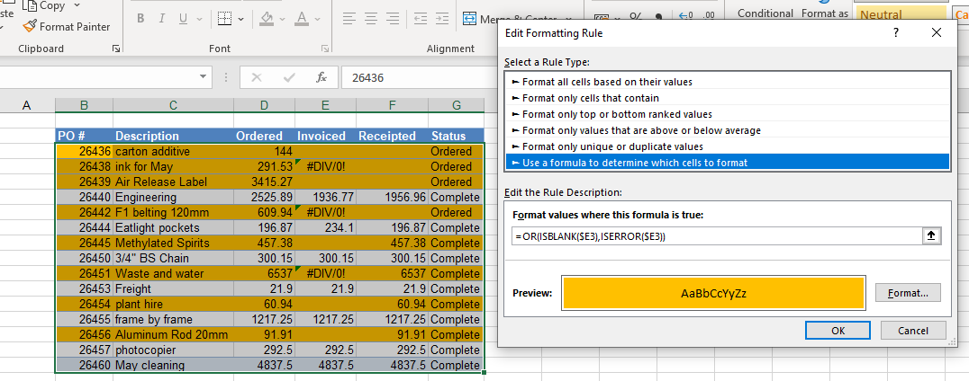
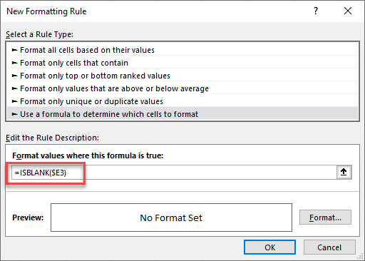
ISBLANK Function

You can use the ISBLANK Function to create a rule to find rows that contain blank or empty cells in the worksheet.

1. Highlight the range and then, in the Ribbon, select Home > Conditional Formatting > New Rule.
2. Type in the formula:
   =ISBLANK($E3)

 

 

3. Click on the Format… button and select your desired formatting and then click OK to return to Excel.

 

 

ISBLANK With OR

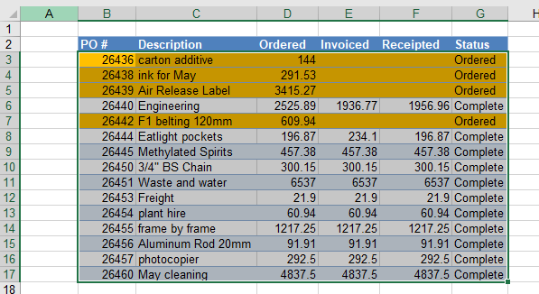
You can expand this to include blank cells or cells with an error in them.

1. Type in the formula
   =OR(ISBLANK($E3),ISERROR($E3))

 

 

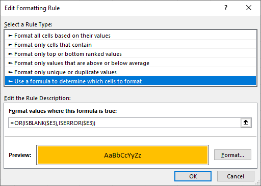
2. Click on the Format… button and select your desired formatting and then click OK to return to Excel.

 

 

Other Functions in Conditional Formatting

There are a variety of other functions that can be used in creating conditional formatting formula-based rules.

• COUNTIFS – counts cells that meet a certain condition (useful for highlighting duplicates)
• LARGE – finds the kth largest value
• MAX – finds the largest number
• MIN – finds the smallest number
• MOD – returns the remainder after division (useful for highlighting every other row)
• NOT – changes TRUE to FALSE and vice versa
• NOW – returns the current date and time (useful for conditionally formatting dates and times)
• ROW – returns the number of rows in an array
• SEARCH – searches for a string of text within another string (useful for finding specific text)
• TODAY – returns the current date (useful for applying conditional formatting to dates)
• VLOOKUP – returns the result of a vertical lookup
• WEEKDAY – returns the day of the week
• XLOOKUP – a new, more powerful lookup function

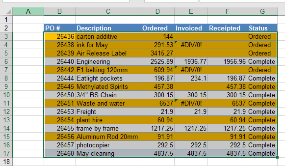
For example, you can use the MAX Function to highlight the row that contains the maximum value in a specified column.

=$D4=MAX($D:$D)

 

 

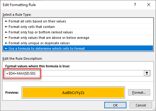
Now, only the row with the maximum value in Column D is highlighted.

 

 

If you are struggling to get a formula to work when creating a conditional formatting rule, it is a good idea to test the formula first in your Excel sheet. Once you have it right there, you can incorporate it in your rule.

Conditional Formatting Based on Formula in Google Sheets

Conditional Formatting works much the same in Google Sheets as it does in Excel.

1. Highlight the cells where you want to set the conditional formatting and then, in the Menu, select Format > Conditional formatting.

 

 

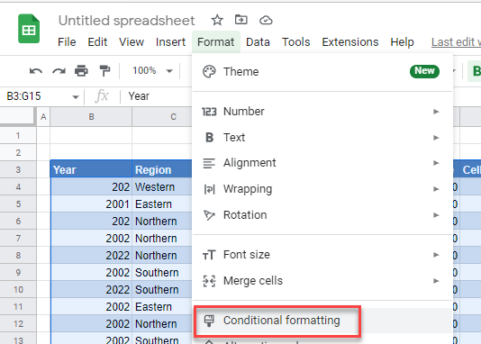
2. Make sure the Apply to range is correct, and then select Custom formula is from the Format rules drop-down box. Type in the formula.

 

 

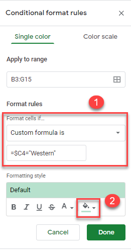
3. Then, select your formatting style and click Done.

 

 

You can also use greater than, greater than or equal to, less than, and less than or equal to in Google Sheets.

AND and OR also work, as well the other functions listed above for Excel (except for XLOOKUP, which does not exist in Google Sheets).