How to Highlight the Highest Value in Excel & Google Sheets

This tutorial demonstrates how to highlight the highest value in a range in Excel and Google Sheets.

 

 

Highlight the Highest Value

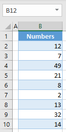
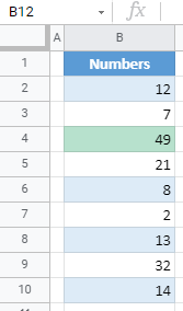
In Excel, you can use conditional formatting to highlight the highest value or the top n values in a range. For this example, let’s start with the data below in Column B.

 

 

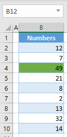
Say you want to highlight the cell with the highest value in green. Since 49 is the highest number in Column B, cell B4 should be highlighted.

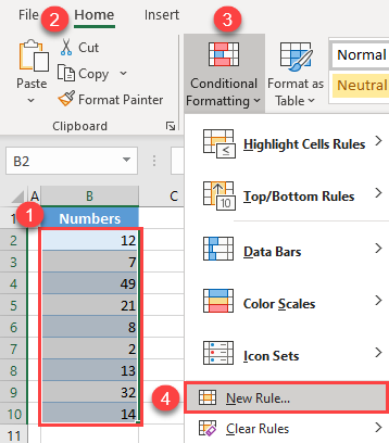
1. Select the data range where you want to highlight the highest value. Then in the Ribbon, go to Home > Conditional Formatting > New Rule…

 

 

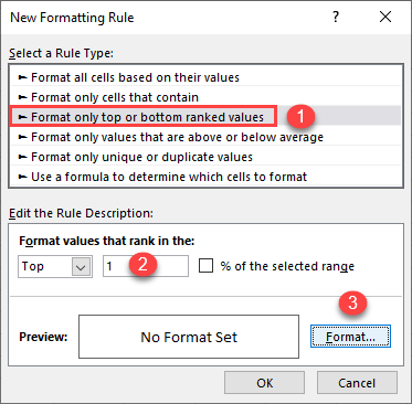
2. In the conditional formatting window, (1) select Format only top or bottom ranked values for Rule Type. Then (2) enter 1 next to Top (as you want one value to be highlighted – the highest), and (3) click Format…

 

 

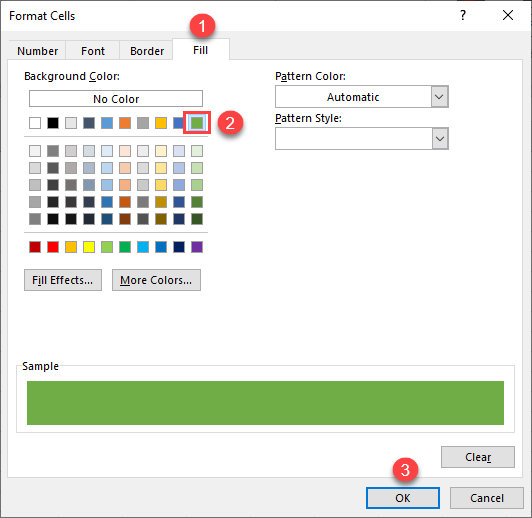
3. In the Format Cells window, (1) go to the Fill tab, (2) choose green and (3) click OK.
   Note that you can also go to the Font, Border, and/or Number tabs to adjust other formatting options.

 

 

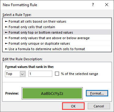
4. Back in the New Formatting Rule window, there’s a Preview of the cell formatting this rule will apply. Click OK.

 

 

Now cell B4 is highlighted green, because 49 is the highest value in the range B2:B10.

 

 

Highlight Top n Values

You can also use conditional formatting to highlight the top n values in a range. Let’s highlight the top three values in the range B2:B10.

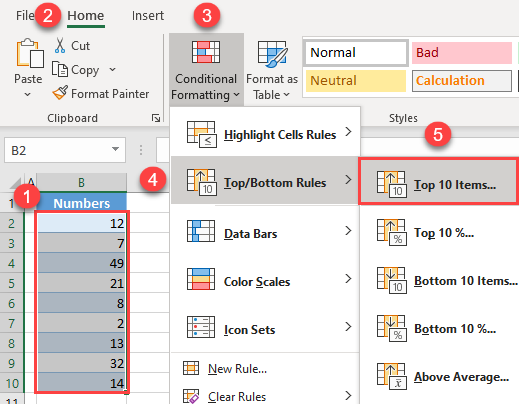
1. Select the data range for which you want to highlight the top three values and in the Ribbon, go to Home > Conditional Formatting > Top/Bottom Rules > Top 10 Items…

 

 

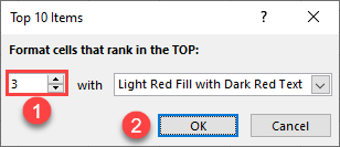
2. The default setting in the pop-up window is to format the top 10 items, but you only want three.
   (1) Enter 3 for the top cells, and (2) click OK, leaving the default formatting (Light Red Fill with Dark Red Text).

 

 

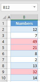
The top three values in the data range (49, 32, and 21) are highlighted.

 

 

If you look back at Step 1, you can see that in the Top/Bottom Rules, there is also an option for Bottom 10 Items. Select that option to highlight the bottom n values in the range.

Highlight the Highest Value in Google Sheets

To highlight the highest value in a range in Google Sheets, follow these steps:

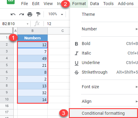
1. Select the data range for which you want to highlight the highest value and in the Menu, go to Format > Conditional formatting.

 

 

2. In the conditional formatting window on the right, (1) choose Custom formula is under Format rules, and (2) enter the formula:

=B2=MAX($B$2:$B$10)

Finally, (3) click OK, leaving the default formatting style (green background fill). This can be changed later by clicking on the Fill color icon.

 

 

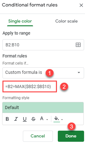
Conditional formatting based on the formula above will be applied if the result of the formula is TRUE. In this case, it’s checking whether each cell in the range is equal to the maximum value in the range (the result of the MAX Function). Since the highest value is in cell B4, the result of the formula for that cell is TRUE, and the B4 cell is highlighted.

 

 

Highlight the Lowest Value in Google Sheets

You can also adjust the formula in Step 2 to highlight the lowest value in a range. To do this, follow the steps for highlighting the highest value above, but use the MIN Function instead:

=B2=MIN($B$2:$B$10)

 

 

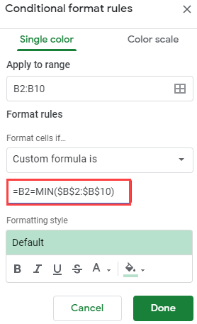
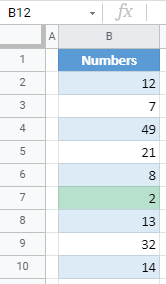
Now, the formula will return TRUE for cell B7, as 2 is the lowest number in the range B2:B10.