COUNTIF and COUNTIFS Functions – Excel, VBA, Google Sheets

This Tutorial demonstrates how to use the ExcelCOUNTIF  and COUNTIFS Functions in Excel to count data that meet certain criteria.

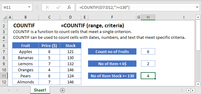
COUNTIF Function Overview

You can use the COUNTIF function in Excel to count cells that contain a specific value, count cells that are greater than or equal to a value, etc.

(Notice how the formula inputs appear)

COUNTIF Function Syntax and Arguments:

=COUNTIF(range, criteria)

range – The range of cells to count.

criteria – The criteria that controls which cells should be counted.

What is the COUNTIF function?

The COUNTIF function is one of the older functions used in spreadsheets. In simple terms, it’s great at scanning a range and telling you how many of the cells meet that condition. We’ll look at how the function works with text, numbers, and dates; as well as some of the other situations that might arise.

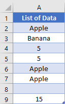
Basic example

Let’s start by looking at this list of random items. We’ve got some numbers, blank cells, and some text strings.

If you wanted to know how many items an exact match to the criteria are, you can specify what you want to look for as the second argument. An example of this formula might look like

=COUNTIF(A2:A9, "Apple")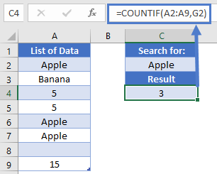

This formula would return the number 3, as there are 3 cells in our range that meet that criteria. Alternatively, we can use a cell reference instead of hardcoding a value. If we wrote “Apple” in cell G2, we could change the formula to

=COUNTIF(A2:A9, G2)

When dealing with number, it’s important to distinguish between numbers and numbers that are been stored as text. Generally, you don’t put quotation marks around numbers when writing formulas. So, to write a formula that checks for the number 5, you would write

=COUNTIF(A2:A9, 5)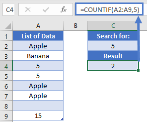

Finally, we could also check for blank cells by using a zero-length string. We would write that formula as

=COUNTIF(A2:A9, "")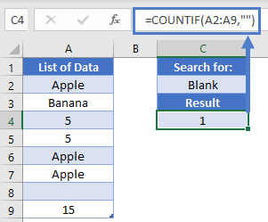

Note: This formula will count both cells that are truly empty, as well as those that are blank as the result of a formula, like an IF function.

Partial matches

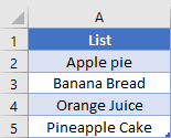
The COUNTIF function supports the use of wildcards, “*” or “?”, in the criteria. Let’s look at this list of tasty bakery goods:

To find all the items that start with Apple, we could write “Apple*”. So, to get an answer of 3, our formula in D2 is

=COUNTIF(A2:A5, "Apple*")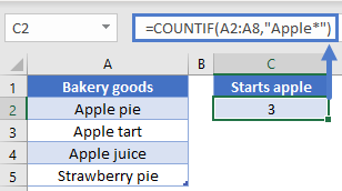

Note: The COUNTIF function is not case-sensitive, so you could also write “apple*” if you want.

Back to our baked goods, we might also want to find out how many pies we have in our list. We can find that by placing the wildcard at the beginning of our search term, and write

=COUNTIF(A2:A5, "*pie")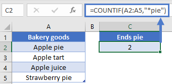

This formula gives the result of 2.

 

We can also use wildcards to check for any cells with text. Let’s go back to our original list of data.

To count the number of cells that have at least some text, thus not counting numbers or blank cell, we can write

=COUNTIF(A2:A9, "*")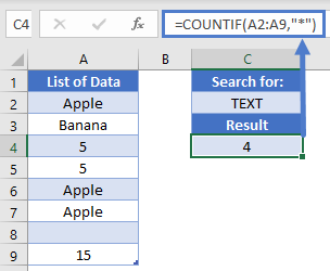

You can see that our formula correctly returns a result of 4.

Comparison operators in COUNTIF

When writing the criteria so far, we’ve been implying that our comparison operator is “=”. In fact, we could have written this:

=COUNTIF(A2:A9, "=Apple")

 

It’s an extra character to write out though, so it’s usually omitted. However, this means that you can use the other operators such as greater than, less than, or not equal to. Let’s look at this list of recorded ages:

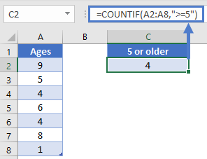
If we wanted to know how many kids are at least 5 years old, we can write out a “greater than or equal to” comparison like so:

=COUNTIF(A2:A8, ">=5")

Note: The comparison operator is always given as a text string, and thus must be inside quotation marks.

Similarly, you can also check for items that are less than a given value. If we need to find out how many are less than 8, we can write out

=COUNTIF(A2:A8, "<8")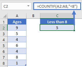

This gives us the desired result of 5. Now let’s imagine that all the 6-year old kids are going on an outing. How many kids will remain? We can figure this out by using a “not equal to” comparison like this:

=COUNTIF(A2:A8, "<>6")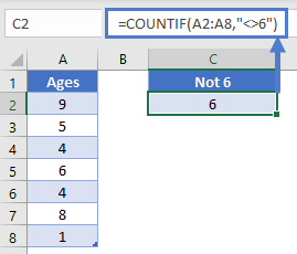

Now we can quickly see that we have 6 kids that are not 6 years old.

In these comparison examples so far, we’ve been hard coding the values we wanted. You can also use a cell reference. The trick is that you need to concatenate the comparison operator with the cell reference. Let’s say that we put the number 7 in cell C2, and we want our formula in D2 to show how many kids are less than 7 years old.

Our formula in D2 needs to look like this:

=COUNTIF(A2:A8, "<"&C2)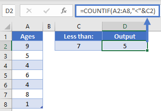

Note: Pay special attention when writing these formulas to whether you need to put an item inside quotation marks, or outside. The operators are always inside quotations, cell references are always outside quotations. Numbers are outside if you’re doing an exact match, but inside if doing a comparison operator.

Working with dates

We’ve seen how you can give a text or number as a criteria, but what about when we need to work with dates? Here’s a quick sample list we can work with:

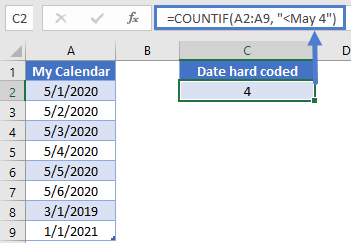
To count how many dates are after May 4, we need to take some caution. Computers store dates as numbers, so we need to make sure the computer uses the right number. If we wrote this formula, would we get the correct result?

=COUNTIF(A2:A9, "<May 4")

The answer is “possibly”. Because we omitted the year from our criteria, the computer will assume we mean the current year. If all the dates we are working with are for the current year, then we’ll get the correct answer. If there are some dates that are in the future however, we’d get the wrong answer. Also, once the next year begins, this formula will return a different result. As such, this syntax should probably be avoided.

Because it can be difficult to write dates correctly within a formula, it’s best practice to write the date you want to use in a cell, and then you can use that cell reference within your COUNTIF formula. So, let’s write the date of 7-May-2020 into cell C2, and then we can put our formula in C4.

The formula in C4 is

=COUNTIF(A2:A9, "<"&C2)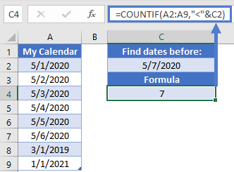

Now we know that the result of 7 is correct, and the answer is not going to change unexpectedly if we open this spreadsheet sometime in the future.

Before we leave this section, it’s common to use the TODAY function when working with dates. We can use that just like we would a cell reference. For instance, we could change the previous formula to be this:

=COUNTIF(A2:A9, "<"&TODAY())

Now our formula will still update as real time progresses, and we will have a count of items that are less than today.

Multiple criteria and COUNTIFS

The original COUNTIF function got an improvement in 2007 when COUNTIFS came out. The syntax between the two is very similar, with the latter allowing you to give additional ranges and criteria. You can easily use COUNTIFS in any situation that COUNTIF exists. It is just a good idea to know that both functions exist.

Let’s look at this table of data:

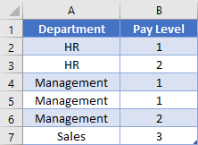
To find out how many people are in pay levels 1 to 2, you could write a summation of COUNTIF functions like this:

=COUNTIF(B2:B7, ">=1")-COUNTIF(B2:B7, ">2")

 

This formula will work, as you’re finding everything that is above 1, but then subtracting the number of records that are beyond your cut-off point. Alternatively, you could use COUNTIFS like this:

=COUNTIFS(B2:B7, ">=1", B2:B7, "<=2")

The latter is more intuitive to read, so you might want to use that route. Also, COUNTIFS is more powerful when you need to consider multiple columns. Let’s say we want to know how many people are in Management and in Pay Level 1. You can’t do that with just a COUNTIF; you’d need to write out

=COUNTIFS(A2:A7, "Management", B2:B7, 1)

This formula would give you the correct result of 2. Before we leave this section, let’s consider an Or type logic. What if we wanted to find out how many people are in Management or? You would need to add some COUNTIFS together, but there are two ways to do this. The simpler way is to write it like this:

=COUNTIF(A2:A7, "HR")+COUNTIF(A2:A7, "Management")

You could also make use of an array, and write this array formula:

=SUM(COUNTIF(A2:A7, {"HR", "Management"}))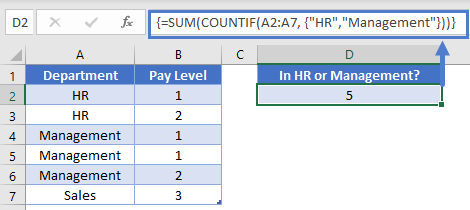

Note: Array formulas must be confirmed using `Ctrl+Shift+Enter` not just `Enter`.

How this formula will work is it will see that you have given an array as the input. It will thus calculate the result to two different COUNTIF functions and store them in an array. The SUM function will then add all the results in our array together to make a single output. Thus, our formula will be evaluated like so:

=SUM(COUNTIF(A2:A7, {"HR", "Management"}))
=SUM({2, 3})
=5

Count unique values

Now that we’ve seen how to use an array with the COUNTIF function, we can take that one step further to help us count how many unique values are in a range. First, let’s look again at our list of Departments.

=SUM(1/COUNTIF(A2:A7,A2:A7))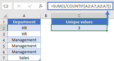

We can see that there are 6 cells worth of data, but there are only 3 different items. To get the math to work out, we’d need each item to be worth 1/N, where N is the number of times an item is repeated. For example, if each HR was only worth 1/2, then when you added them up you would get a count of 1, for 1 unique value.

Back to our COUNTIF, which is designed to figure out how many times an item appears in a range. In D2, we’ll write the array formula

=SUM(1/COUNTIF(A2:A7, A2:A7))

How this formula will work, is for each cell in the range of A2:A7, it will check to see how many times it appears. With our sample, this is going to produce an array of

{2, 2, 3, 3, 3, 1}

 

Then, we turn all those numbers into fractions by doing some division. Now our array looks like

{1/2, 1/2, 1/3, 1/3, 1/3, 1/1}

 

When we add these all up, we get our desired result of 3.

Countif with Two or Multiple Conditions – The Countifs Function

So far we’ve worked only with the COUNTIF Function. The COUNTIF Function can only handle one criteria at a time. To COUNTIF with multiple criteria you need to use the COUNTIFS Function. COUNTIFS behaves exactly like COUNTIF. You just add extra criteria. Let’s take a look at below example.

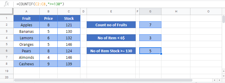
=COUNTIFS(B2:B7,"<6",C2:C7,">=130")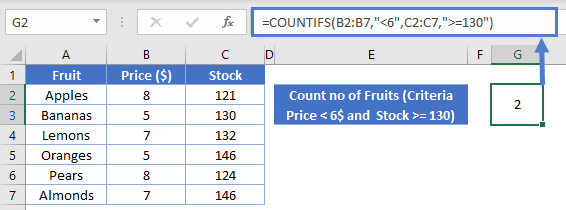

COUNTIF & COUNTIFS in Google Sheets

The COUNTIF & COUNTIFS Function works exactly the same in Google Sheets as in Excel: