Conditionally Format Dates and Times in Excel & Google Sheets
Written by
Reviewed by
This tutorial will demonstrate how to conditionally format dates and times in Excel.
Conditional Formatting
Conditional Formatting will format cells IF certain conditions are met. To access Conditional Formatting go to Home > Conditional Formatting.
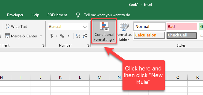
Next Click “New Rule”. We will use the option ‘Use a formula to determine which cells to format’:
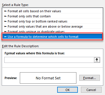
In today’s examples, we will be using formulas to conditionally format our cells as they are the most customizable. A summary of the rule types can be seen below (we are using a hypothetical data set of test scores as an example).
| Rule Type | Use | Example |
| Format all cells based on their values | If you want to create a visual representation of minimum and maximum values in either a color scheme format or a data bar format. | You want to show test scores so that the highest marks are green and the lowest marks are red. The lower the mark, the redder that cell is. |
| Format only cells that contain | If you want to highlight cells that contain a specific word or value | You want to only highlight cells that have a test score value of over 90, or, you want to only highlight cells that have a specific name of a test candidate. |
| Format only top or bottom ranked values | If you want to highlight cells which are the highest in a range | You want to highlight the top 10% of the test scores. |
| Format only values that are above or below above average | If you want to highlight cells that are above or below the average | You want to highlight any scores below the average. |
| Format only unique or duplicate values | If you want to highlight cells that are either unique or duplicates | You want to only highlight test candidate names that were duplicated. |
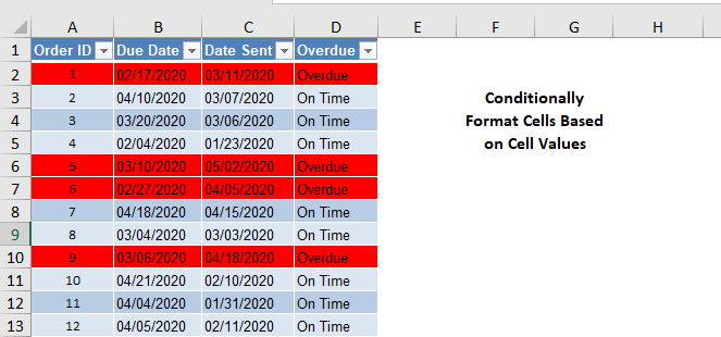
Conditional Format Cell If Date Is Overdue
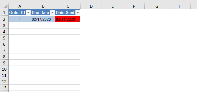
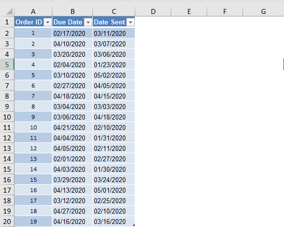
In the data set above, we can see that cell C2 is highlighted because cell C2 is greater than cell B2 meaning that the Order ID is overdue. To do this, we will first select cell C2, then click on “Conditional Format”, “New Rule” and then navigate to “Use a formula to determine which cells to format” as we saw above. In the formula bar where it says “Format values where this formula is true”, we will enter the formula “=C2>B2”. We will then format this to be red in colour as seen below.
Remember to always select the range you want conditionally formatted before entering in any formulas
You will notice that this is a TRUE/FALSE statement. If the statement is TRUE, then the condition will be met, allowing for the format to occur, hence why it’s called “Conditional Formatting”.
Conditional Format Row If Date is Overdue
In real data sets, you will be working with multiple rows of data and so setting conditional formats for multiple rows is not feasible. You can conditionally format an entire row based on the value of another cell with the use of absolute references. In the example above, let’s say you want to conditionally format all rows that are overdue.
Navigate back to the Conditional Formatting formula rule type. Select the range from A2 to B20.
You will notice I have not included the column headers. Only include the data set that you want conditionally formatted and nothing else. This will allow Microsoft Excel/Google Sheets to understand which data set you are trying to visually represent.
In the formula bar where it says “Format values where this formula is true”, we will enter the formula “=$C2>$B2”.
The “$” sign is known as an absolute reference. An absolute reference allows for references to not change when a formula is copied down and/or across.
For conditional formatting, adding a $ sign to the left of the column ID will mean the conditional formatting will apply to the row.
Using the formula above, you will see that all rows that are overdue have been highlighted in red.
Conditional Format Row Based On Text Value
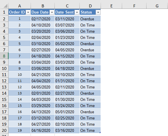
Using the same concept, we can also conditionally format rows based on text values. In the same data set, we have added another column for orders that are “Overdue” and “On Time” to demonstrate this.
Navigate back to the Conditional Formatting formula rule type. Select the range from A2 to B20.
In the formula bar where it says “Format values where this formula is true”, we will enter the formula “=$D2=’Overdue'”

In this case, we have used text rather than a cell reference in order to determine which items are overdue.

