XLOOKUP Text – Excel & Google Sheets

This tutorial will demonstrate how to use the XLOOKUP Function with text in Excel.

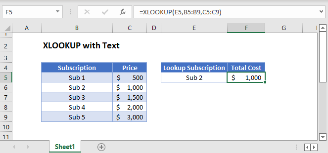
XLOOKUP with Text

To lookup a string of text, you can enter the text into the XLOOKUP Function enclosed with double quotations.

=XLOOKUP("Sub 2",B3:B7,C3:C7)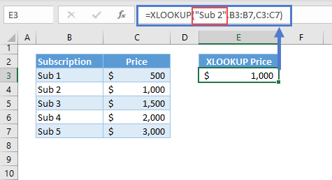

XLOOKUP with Text in Cells

Or, you can reference a cell that contains text.

=XLOOKUP(E3,B3:B7,C3:C7)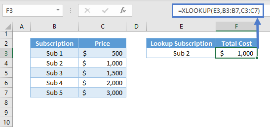

XLOOKUP with Multiple Texts

If you want to look up a series of texts, enter the range reference into the formula, and a dynamic array “Spill” formula will be created.

=XLOOKUP(E3:E4,B3:B7,C3:C7)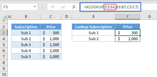

The formula will “spill” to perform the calculations on the entire array of values.

 

Alternatively, you can reference a single cell, lock cell references, and copy the formula down.

=XLOOKUP(E3,$B$3:$B$7,$C$3:$C$7)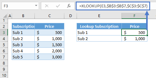

Note: Make sure that the 2^nd and 3^rd arguments are in absolute references by adding dollar signs in front of the Column Letter and Row Number (or you can put the cursor in the reference while in the formula and press F4). This will fix the references while you’re dragging or copying the formula.

XLOOKUP with Last Text

By default, the XLOOKUP Function will search an exact match from the top of the list going down (i.e., Top-Down approach). We can reverse this by applying a value of -1 to the last argument: search_mode.

We can find the last occurrence of a text within a list by applying -1 to the last argument of the XLOOKUP Function.

=XLOOKUP(E3,B3:B7,C3:C7,,,-1)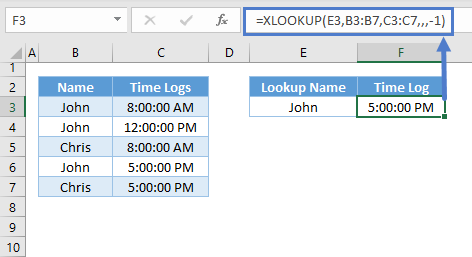

XLOOKUP with EXACT Function

It’s not obvious from the previous examples, but the matching process of the XLOOKUP Function is case-insensitive. This means that text will match regardless of case (upper or lower).

We can use the EXACT Function to perform a case-sensitive match.

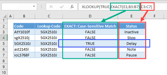
=XLOOKUP(TRUE,EXACT(E3,B3:B7),C3:C7)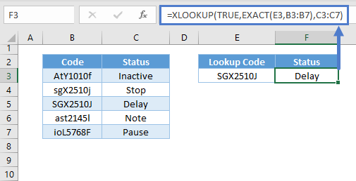

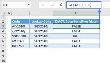
Let’s visualize how the formula above works:

The EXACT Function performs a case-sensitive comparison between two values.

In our example, an array is created, comparing the lookup value (see Column C) and each of the values from the lookup array (see Column B). The EXACT Function will return TRUE if the texts being compared are the same and FALSE if different (see Column D).

In our XLOOKUP Formula it looks like this:

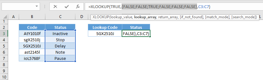
Note: This will only work if there’s an array input (B3:B7 in the XLOOKUP formula). The EXACT Function will also return an array output as visualized in Column D.

The array output of the EXACT Function is then used as the lookup array for the XLOOKUP Function. We’ll search for the first occurrence of the TRUE value, which means an exact match, and return the corresponding status.

 

XLOOKUP with Partial Match

The matching process in the previous examples are all done by matching whole texts or phrases, but we can also perform a partial match in XLOOKUP.

XLOOKUP with Wildcards

The easiest method to perform a partial match is to use wildcards. We need to change the 5^th argument: match_mode to 2 to enable this.

=XLOOKUP("*"&E3&"*",B3:B7,C3:C7,,2)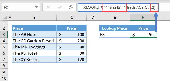

Note: The asterisk wildcard represents any number of any characters. By adding the asterisk to the front and end, we search for any text that contains “RS”.

XLOOKUP with SEARCH Function

Another way to perform a partial match is to nest a SEARCH Function inside the XLOOKUP.

In order for this to work, we must enclose the SEARCH Function using the ISNUMBER Function.

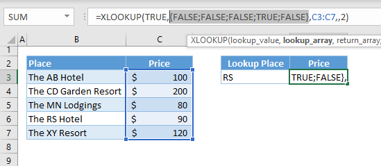
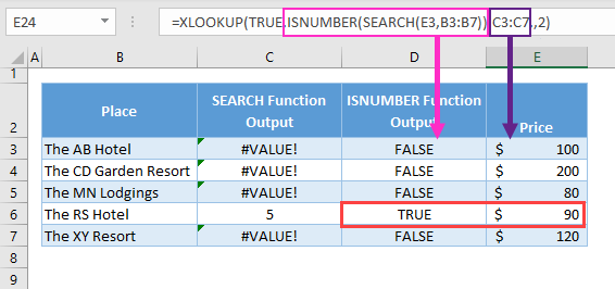
=XLOOKUP(TRUE,ISNUMBER(SEARCH(E3,B3:B7)),C3:C7,,2)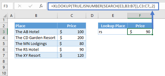

Let’s visualize how the formula works:

The SEARCH Function searches a text from another text. It will return a position number if it finds the lookup text. Otherwise, it will return an error.

Since we have an array input (B3:B7), it will perform the search for each of the values within the input array and will return an array output (Column C below).

 

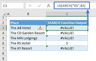
Here’s how it looks in our formula:

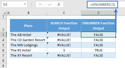
The array output from the SEARCH Function is then feed to the ISNUMBER Function, which checks if the returned values of the SEARCH Function are numbers. If a value is a number, it will return TRUE. Otherwise, FALSE. (Please see Column D below)

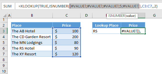
Here’s how the result of the ISNUMBER looks in the formula:

We now have an array output of TRUE and FALSE values, which are used as the lookup array for the XLOOKUP Function. We’ll lookup for TRUE as the partial match.

 

XLOOKUP with FIND Function

The SEARCH and FIND Functions are almost the same function. One important difference is that the SEARCH Function is case-insensitive while the FIND Function is case-sensitive.

To perform a case-sensitive partial match, we’ll use the combination of the FIND Function and the ISNUMBER Function.

=XLOOKUP(TRUE,ISNUMBER(FIND(E3,B3:B7)),C3:C7,,2)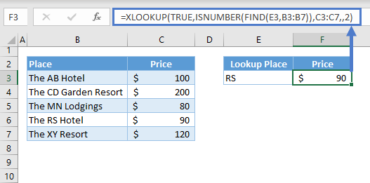

XLOOKUP Partial Match Problem

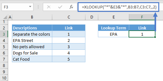
The previous partial matching methods discussed in the previous sections have one major flaw. They can’t distinguish an exact text match within a given phrase.

The partial matching process below can’t distinguish the term EPA to the “epa” from the word “Separate.”

 

XLOOKUP Exact Partial Match

If the words are separated by spaces, then we can add spaces to perform an exact partial match.

=XLOOKUP("* "&E3&" *"," "&B3:B7&" ",C3:C7,,2)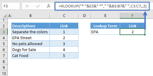

Note: We add spaces before and after E3, and we also do the same for the lookup array in B3:B7. This will bound the words with spaces at their front and end, which will be used to distinguish an exact matching of term within the phrases.

 

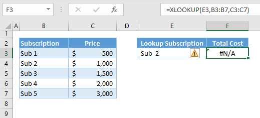
XLOOKUP Text Problem

One of the most common problems in text matching are unwanted spaces. Spaces are treated as part of texts. Therefore, if there are extra spaces, which are hard to notice, the XLOOKUP Function will return an error. Make sure that there are no unwanted spaces within the lookup value and the lookup array.

The lookup value (E3) in the example below has an extra space between the “Sub” and “2.”

XLOOKUP with TRIM Function

We can use the TRIM Function to solve the extra spaces. We can apply it to both the lookup value and the whole lookup array.

=XLOOKUP(TRIM(E3),TRIM(B3:B7),C3:C7)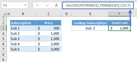

Note: The TRIM Function removes extra spaces between words until there’s a one space boundary between them, and any spaces before the first word and after the last word of a text or phrase are removed.