SEARCH Fx – Find Substring in String – Excel, VBA & G Sheets

This tutorial demonstrates how to use the SEARCH Function in Excel and Google Sheets to locate the position of text within a cell.

What Is the SEARCH Function?

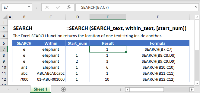
The Excel SEARCH Function “searches” for a string of text within another string. If the text is found, SEARCH returns the numerical position of the string.

Note: SEARCH is NOT case-sensitive. This means “text” will match “TEXT”. To search text with case-sensitivity use the FIND Function instead.

How to Use the SEARCH Function

The Excel SEARCH Function works in the following way.

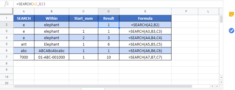
=SEARCH("e", B3)

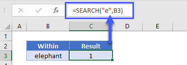
Here, Excel will return 1, since “e” is the first character in “elephant”.

Below are a few more examples.

Start Number (start_num)

Optionally, you can define a Start Number (start_num). start_num tells the SEARCH function where to start the search. If you leave it blank, the search will start at the first character.

=SEARCH(B3,C3)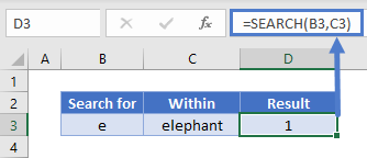

Now, let’s set start_num to 2, which means SEARCH will start looking from the second character.

=SEARCH(B3,C3,D3)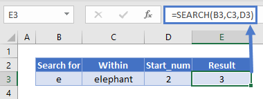

In this case, SEARCH returns 3: the position of the second “e”.

Important: start_num has no impact on the return value, SEARCH will always start counting with the first character.

Start Number (start_num) Errors

If you do use a start number, make sure it’s a whole, positive number that’s smaller than the length of the string you want to search, otherwise you’ll get an error. You’ll also get an error if you pass a blank cell as your start number:

=SEARCH(B3,C3,D3)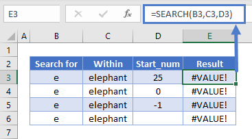

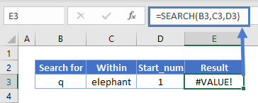
Unsuccessful Searches Return a #VALUE! Error

If SEARCH can’t find the search value, Excel will return a #VALUE! error.

 

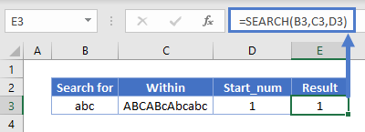
Case-Insensitive Search

The example below demonstrates that the SEARCH function is case-insensitive. We searched for “abc”, but SEARCH returned 1, because it matched “ABC”.

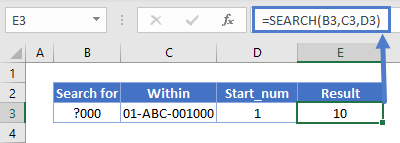
Wildcard Search

You can use wildcards with SEARCH, which enable you to search for unspecified characters.

A question mark in your search text means “any character”. So “?000” in the example below means “Search for any character followed by three zeroes.”

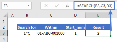
An asterisk means “any number of unknown characters”. Here we’re searching for “1*C”, and SEARCH returns 2 because it matches that with “1-ABC”.

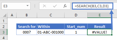
In the next example, we’re searching for “000?” – that is, “000” followed by any character. We have “000”, but it’s at the end of the string, and therefore isn’t followed by any characters, so we get an error

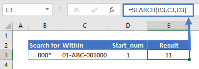
However, if we used an asterisk instead of a question mark – so “000*” instead of “000?”, we get a match. This is because the asterisk means “any number of characters” – including no characters.

How to Split First and Last Names from a Cell with SEARCH

If you have first and last names in the same cell, and you want to give them a cell each, you can use SEARCH for that – but you’ll need to use a few other functions too.

Getting the First Name

The LEFT Function returns a certain number of characters from a string, starting from the left.

If we use SEARCH to return the position of the space between the first and last name, subtract 1 from that, we know how long the first name is. Then we can just pass that to LEFT.

The first name formula is:

=LEFT(B3,SEARCH(“ “,B3)-1)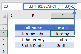

Getting the Last Name

The RIGHT Function returns a certain number of characters from the right of a string.

To get a number of characters equal to the length of the last name, we use SEARCH to tell us the position of the space, then subtract that number from the overall length of the string – which we can get with LEN.

The last name formula is:

=RIGHT(B3,LEN(B3)-SEARCH(“ “,B3))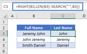

Note that if your name data contains middle names, the middle name will be split into the “Last Name” cell.

Using SEARCH to Return the nth Character in a String

As noted above, SEARCH returns the position of the first match it finds. But by combining it with CHAR and SUBSTITUTE, we can use it to locate later occurrences of a character, such as the second or third instance.

Here’s the formula:

=SEARCH(CHAR(134),SUBSTITUTE(D3,C3,CHAR(134),B3))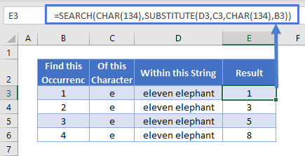

It might look a little complicated at first, so let’s break it down:

• We’re using SEARCH, and the string we’re searching for is “CHAR(134)”. CHAR returns a character based on its ASCII code. CHAR(134) is a dagger symbol – you can use anything here as long it doesn’t appear in your actual string.
• SUBSTITUTE goes through a string and replaces one character or substring for another. Here, we’re substituting the string we want to find (which is in C3) with CHAR(134). The reason this works, is that SUBSTITUTE’s fourth parameter is the instance number, which we’ve stored in B3.
• So, SUBSTITUTE swaps the nth character in the string for the dagger symbol, and then SEARCH returns the position of it.

Here’s what it looks like:

 

Finding the Middle Section of a String

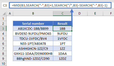
Imagine you have many serial numbers with the following format:

AB1XCDC-1BB/BB99

You’ve been asked to pull out the middle section of each one. Rather than doing this by hand, you can combine SEARCH with MID to automate this task.

The MID Function returns a portion of a string. Its inputs are a text string, a start point, and a number of characters.

Since the start point we want is the character after the hyphen, we can use SEARCH to get the hyphen’s position, and add 1 to it. If the serial number was in B3 we’d use:

=SEARCH("-",B3)+1

To get the number of characters we want to pull out from here, we can use search to get the position of the forward slash, subtract the position of the hyphen, and then subtract 1 so ensure we don’t return the forward slash itself:

=SEARCH("/",B3)-SEARCH("-",B3)-1

Then we simply plug these two formulas into MID:

 

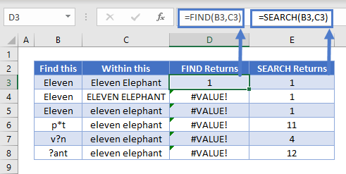
SEARCH Vs FIND

SEARCH and FIND are similar functions. They both return the position of a given character or substring within another string. However, there are two key differences:

• FIND is case sensitive but SEARCH is not
• FIND does not allow wildcards, but SEARCH does

 

You can see a few examples of these differences below:

 

SEARCH in Google Sheets

The SEARCH Function works exactly the same in Google Sheets as in Excel:

Additional Notes

The SEARCH Function is a non case-sensitive version of the FIND Function. SEARCH also supports wildcards. Find does not.

SEARCH Examples in VBA

You can also use the SEARCH function in VBA. Type:

application.worksheetfunction.search(find_text,within_text,start_num)

For the function arguments (find_text, etc.), you can either enter them directly into the function, or define variables to use instead.

Return to the List of all Functions in Excel