Introduction to Dynamic Array Formulas in Excel
Written by
Reviewed by
Download the example workbook
This tutorial will give you Introduction to Dynamic Array Formulas in Excel and Google Sheets.
Introduction
In September 2018 Microsoft introduced Dynamic Array Formulas to Excel. Their purpose is to make it easier to write complex formulas and with less chance of error.
Dynamic Array Formulas are meant to eventually replace Array Formulas, i.e. advanced formulas that require the use of Ctrl + Shift + Enter (CSE).
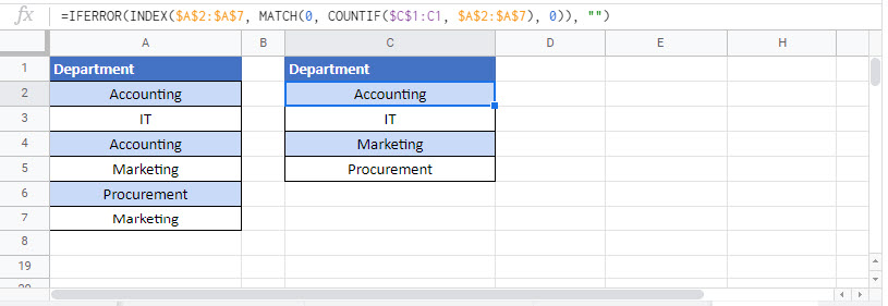
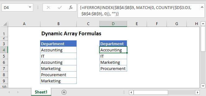
Here’s a quick comparison between the Array Formula and Dynamic Array Formula used to extract a list of unique departments from our list in range A2:A7.
Legacy Array Formula (CSE):
The following formula is input in the cell D2 and is entered by hitting Ctrl + Shift + Enter and copying it down from D2 to D5.
{=IFERROR(INDEX($A$2:$A$7, MATCH(0, COUNTIF($D$1:D1, $A$2:$A$7), 0)), "")}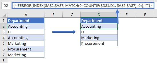
Dynamic Array Formula:
The following formula is only input in the cell D2 and entered by hitting Enter. From a quick glance you can tell how easy and straight-forward it is to write a Dynamic Array Formula.
=UNIQUE(A2:A7)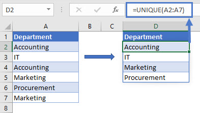
Availability
As of August 2020, Dynamic Array Formulas are only available to Office 365 Users.
Spill and Spill Range
Dynamic Array Formulas work by returning multiple results to a range of cells based on a single formula entered in one cell.
This behavior is referred to as “Spilling” and the range of cells where the results are placed is called the “Spill Range”. When you select any cell within the spill range, Excel highlights it with a thin blue border.
In the example below, the dynamic array formula SORT is in cell D2 and the results have been spilled in the range D2:D7
=SORT(A2:A7)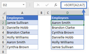
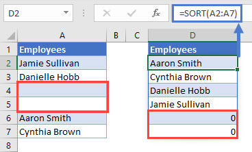
The results of the formula are dynamic which means if a change occurs in the source range, the results also change and the spill range resizes.
#SPILL!
You should note that if your Spill Range is not completely blank, a #SPILL error is returned.
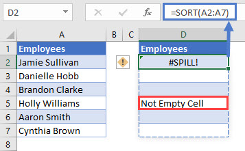
When you select the #SPILL error, the formula’s desired Spill Range is highlighted with a dashed blue border. Moving or deleting the data in the non-blank cell removes this error allowing the formula to spill.
Spill Reference Notation
To reference a formula’s spill range we place the # symbol after the cell reference of the first cell in the spill.
You can also reference the spill by selecting all cells in the spill range and a reference to the spill will be automatically created.
In the example below we’d like to count the number of employees in our firm using the formula COUNTA after they have been ordered alphabetically using the dynamic array formula SORT.
We enter the SORT formula in D2 to order the employees in our list:
=SORT(A2:A7)
We then enter the COUNTA formula in G2 to count the number of employees:
=COUNTA(D2#)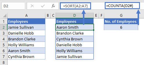
Note the use of # in D2# to refer to the results spilled by SORT in range D2:D7.
New Formulas
Below is the full list of the new Dynamic Array Formulas:
- UNIQUE – Returns a list of unique values from a range
- SORT – Sorts values in a range
- SORTBY – Sorts values based on a corresponding range
- FILTER – Filters a range based on the provided criteria
- RANDARRAY – Returns an array of random numbers between 0 and 1
- SEQUENCE – Generates a list of sequential numbers such as 1, 2, 3, 4, 5
Dynamic Array Formulas in Google Sheets
All of the above examples work exactly the same in Google Sheets as in Excel.