Highlight Blank Cells -Conditional Formatting

This tutorial will demonstrate you how to highlight blank cells using Conditional Formatting in Excel and Google Sheets

Highlight Blank Cells with Conditional Formatting – ISBLANK Function

To highlight blank cells with conditional formatting, you can use the ISBLANK Function within a Conditional Formatting rule.

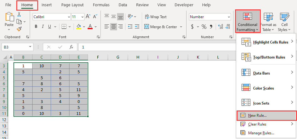
1. Select the range to apply the formatting (ex. B3:E11)
2. In the Ribbon, select Home > Conditional Formatting > New Rule.

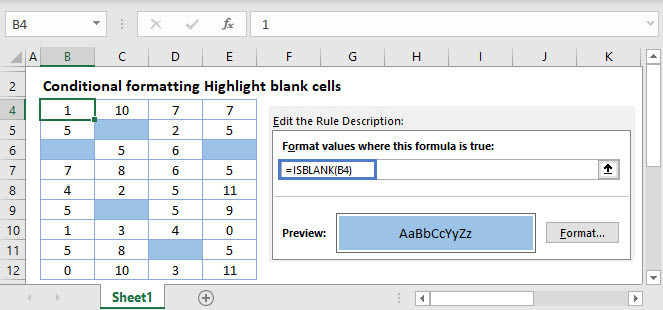
3. Select “Use a formula to determine which cells to format‘, and enter the following formula:

=ISBLANK(B3)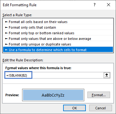

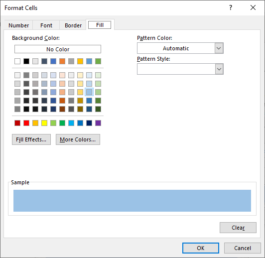
4. Click on the Format button and select your desired formatting.

5. Click OK, and then OK once again to return to the Conditional Formatting Rules Manager.
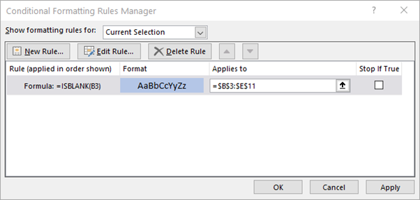
6. Click Apply to apply the formatting to your selected range and then click Close.

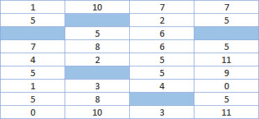
Now your range is conditionally formatted if blank cells are detected:

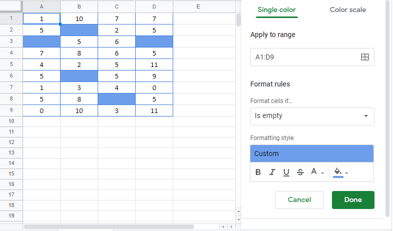
Google Sheets –Highlight Blank Cells (Conditional Formatting)

All of the above examples work exactly the same in Google Sheets as in Excel.