Apply Conditional Formatting Based on Adjacent Cell in Excel & Google Sheets

In this tutorial, you will learn how to apply conditional formatting based on the contents of an adjacent cell in Excel and Google Sheets.

 

 

Apply Conditional Formatting Based on an Adjacent Cell

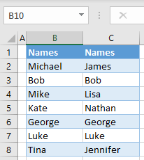
In Excel, you can compare two adjacent cells and apply conditional formatting based on the comparison. For the following example, let’s start with two lists of names (in Columns B and C).

 

 

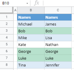
Say you want to highlight (in green) all cells where a cell from Column B has the same value in Column C.

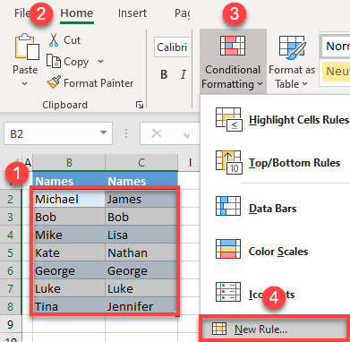
1. Select a range of data and in the Ribbon, go to Home > Conditional Formatting > New Rule.

 

 

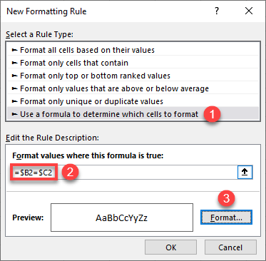
2. In the New Formatting Rule window, (1) select Use a formula to determine which cells to format. In the formula box, (2) enter the formula:

=$B2=$C2

Now (3) click Format. The formula will go row-by-row (down Columns B and C, fixed by the absolute references in the formula) and compare values. If they are equal, the formatting will be applied.

 

 

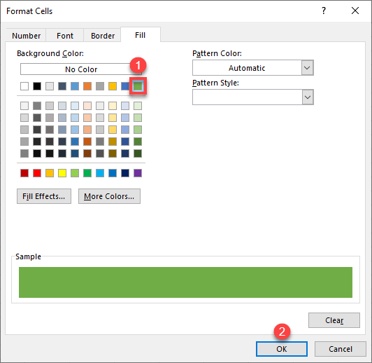
3. In the Format Cells window, choose a color (here, green), and click OK.

 

 

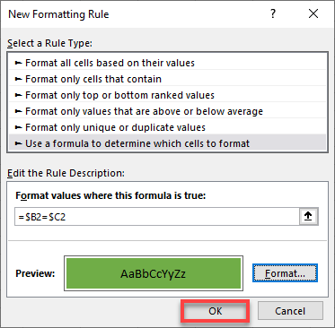
4. This takes you back to the New Formatting Rule window; click OK. Before clicking OK, you can Preview and check the formatting.

 

 

As a result, all cells that have matching values in Columns B and C are colored green (B3, B6, and B7).

 

 

Apply Conditional Formatting Based on an Adjacent Cell in Google Sheets

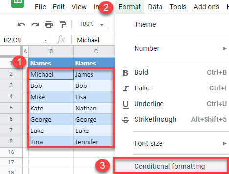
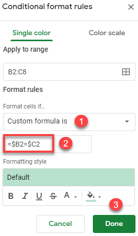
1. Select a range of data and in the Menu, go to Format > Conditional formatting.

 

 

2. In the Conditional format rules window on the right, choose Custom formula is, enter the formula:

=$B2=$C2

Then click Done. This leaves the default formatting (green background color), but if you want to change that, just click on the Fill icon.

 

 

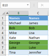
Finally, the result is the same as in Excel: All cells with matching values in Columns B and C are green.