How to Alternate Row Color in Excel & Google Sheets

This tutorial demonstrates how to alternate row color in Excel and Google Sheets.

Alternate Row Color

Table Formatting

To format a table with alternating row colors, you can use the Format as Table feature in Excel.

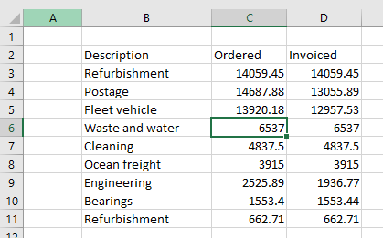
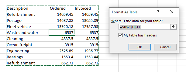
1. Select the cells you wish to apply the alternating row colors (or click in the range with your table).

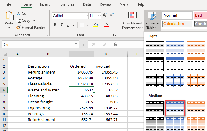
2. Then in the Ribbon, go to Home > Styles > Format as Table. Choose an alternating row style from the formatting options.

3. If applicable, check My table has headers. Click OK.

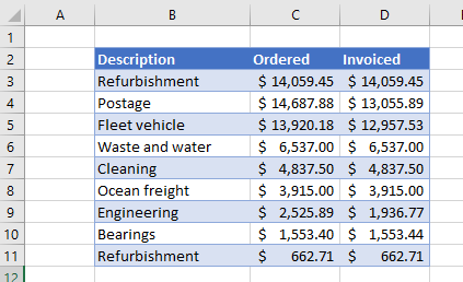
The data is formatted as a table with alternating row colors.

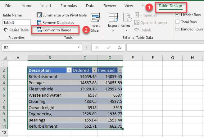
4. Notice there is a new Table tab on the Ribbon.
   Click Convert to Range to convert the table back into a simple range of cells.

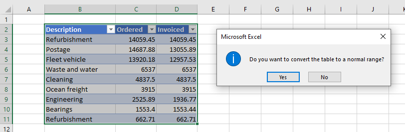
5. Click OK to convert the table to a normal range.

Insert Tab

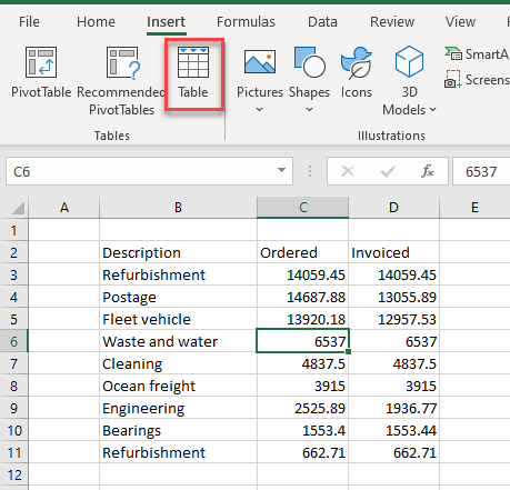
Another way to format data as a table (Steps 1–3 above) is through the Ribbon’s Insert tab.

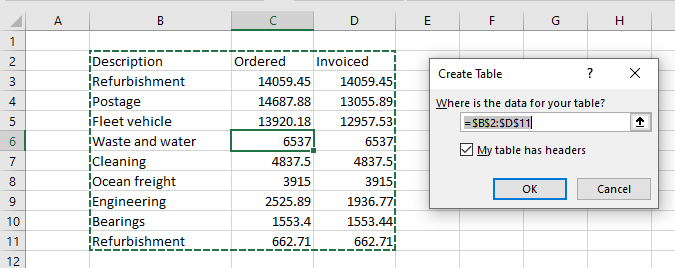
1. In the Ribbon, go to Insert > Table.

2. Once again, check the My table has headers checkbox if relevant.

Conditional Formatting

You can also create alternating colors for each row using conditional formatting.

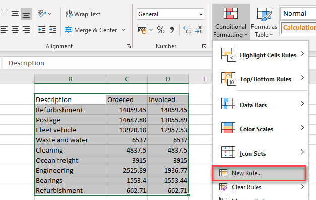
1. Select the cells you wish to apply the alternating row colors to, and then in the Ribbon, go to Home > Styles > Conditional Formatting > New Rule…

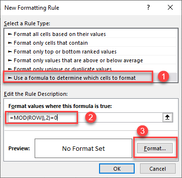
2. In the New Formatting Rule dialog box, click Use a formula to determine which cells for format.
   Then, type in the formula:

   =MOD(ROW(),2)=0

   Click Format…

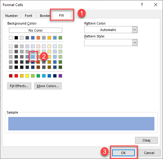
3. In the Format Cells dialog box, go to the Fill tab and choose a Background Color. Click OK, and then click OK again to return to Excel.

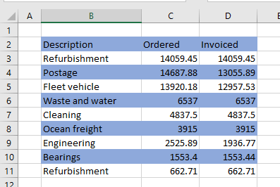
As you can see below, the data has alternating colors.

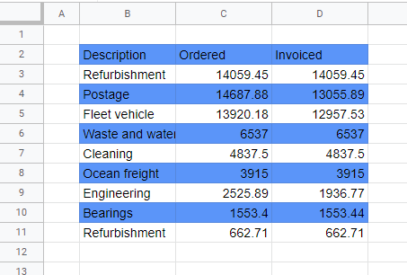
Alternate Row Color in Google Sheets

Alternating Colors

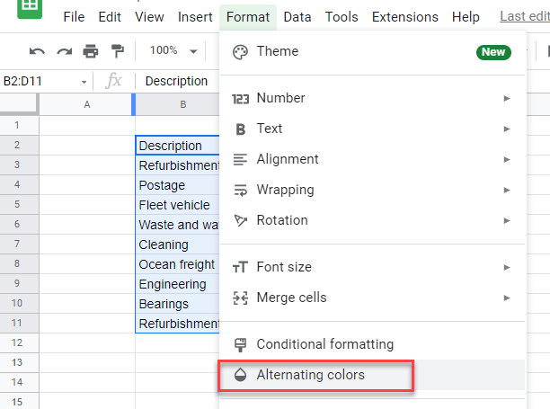
1. Select the cells you wish to apply the alternating row colors or click in the middle of the range of cells you wish to apply the alternating row colors to.
2. In the Menu, go to Format > Alternating colors.

3. This sets the entire table (B2:D11) as the Apply to range.
   Under Styles, Header is automatically ticked – you can remove the checkmark if you don’t need a header row.
   Choose a style from Default styles, or create a Custom style and pick your own colors for the header and alternate rows.

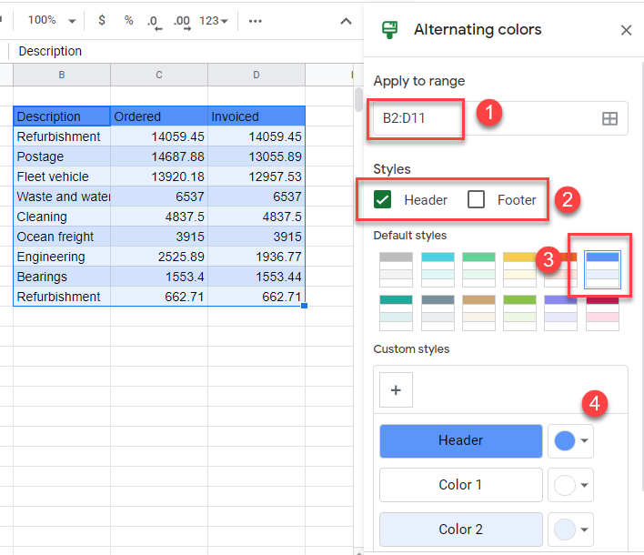
4. Click Done to apply the format to the Google Sheet.

Conditional Formatting

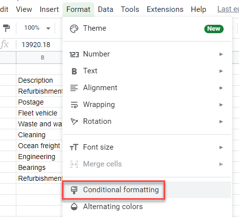
You can also apply alternating colors in Google Sheets using conditional formatting.

Select the cells you wish to format, and then in the Menu, go to Format > Conditional formatting.

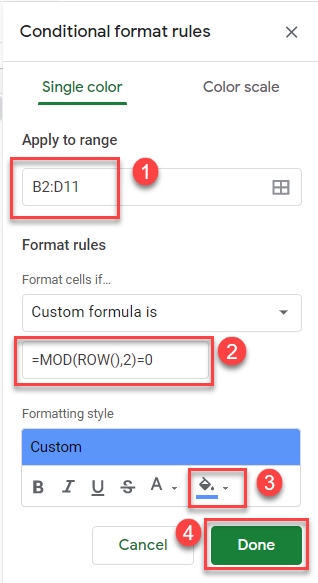
1. Select the range, and then under Format rules, Format cells if… Custom formula is.
2. Use the custom formula from the Excel example above.

   =MOD(ROW(),2)=0

3. Choose a fill color for the cells.
4. Then click Done.

Again, you get alternating colors.