Conditional Formatting – Highlight Entire Row in Excel & Google Sheets

This article will demonstrate how to use conditional formatting to highlight an entire row in Excel and Google Sheets.

 

 

A row can be highlighted based on the contents of one cell in that row by using Excel’s Conditional Formatting feature.

Highlight Entire Row

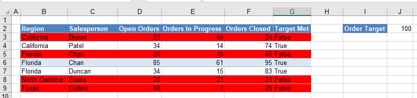
Say you want to check whether a sales target is met or not. You can create a formula to return either TRUE or FALSE in your worksheet based on the values contained in your worksheet.

 

 

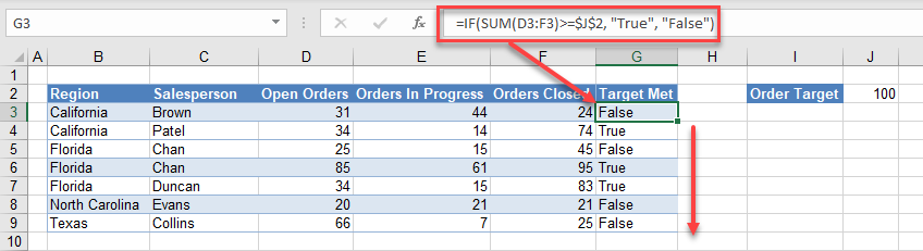
In the example above, an IF statement tests whether the sum of the orders is greater than or equal to 100.

=IF(SUM(D3:F3)>=$J$2,”True”,”False”)

If the sum of the orders is greater than or equal to 100, then TRUE is returned by the IF Function, otherwise FALSE is returned.

To see at a glance if the order target has been met, you can then apply a conditional formatting rule to the worksheet.

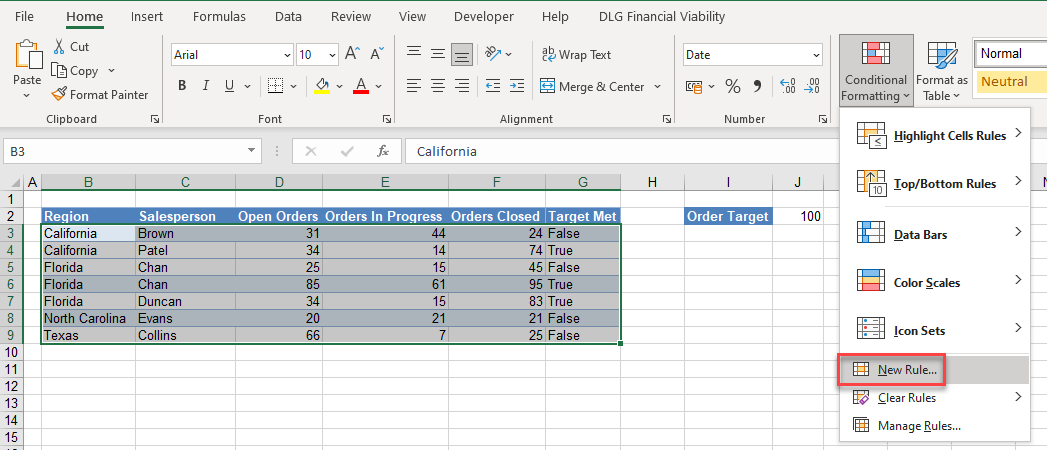
1. Highlight the rows to be formatted, and then in the Ribbon, select Home > Styles > Conditional Formatting > New Rule…

 

 

2. Select Use a formula to determine which cells to format, and enter the formula:
   =$G3=”FALSE”

 

 

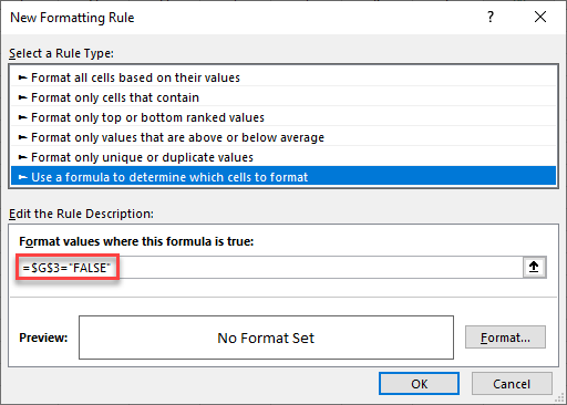
You need to use a mixed reference in this formula ($G3) in order to lock the column but make the row relative. This enables the formatting to format the entire row instead of just a single cell that meets the criteria.
When the rule is evaluated for all the cells in the range, the row changes but the column does not. This causes the rule to ignore the values in any of the other columns and just concentrate on the values in Column G. As long as the rows match, and Column G of that row contains the word FALSE, then the formula result is TRUE and the formatting is applied for the whole row.

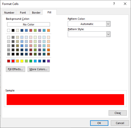
3. Click on the Format button and select your desired formatting.

 

 

4. Click OK and then OK again to view the result.

 

 

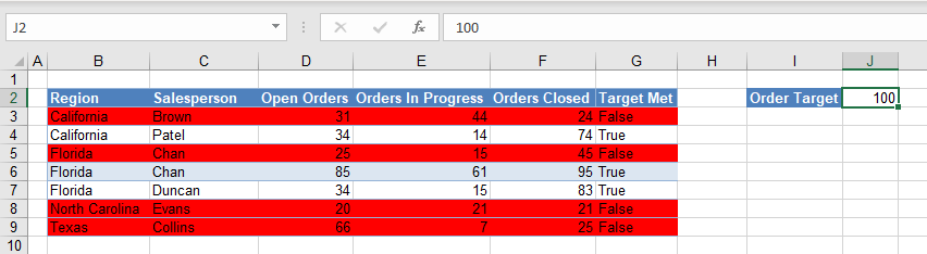
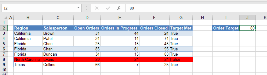
Now, if you change the order target (here, J2), the cell format also changes.

 

 

Highlight Entire Row in Google Sheets

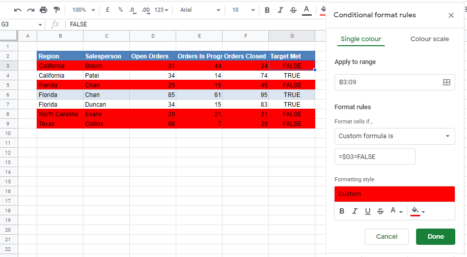
Using conditional formatting to highlight an entire row in Google Sheets is similar.

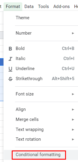
1. Highlight the rows you wish to format, and go to Format > Conditional Formatting.

 

 

2. The Apply to range section is already filled in. Select Custom formula is, and then type in the formula:
   =$G3=FALSE
   Once again, you need to use a mixed reference to make the column, but not the row, absolute.
3. Select a formatting style, and then click Done.