How to Compare Two Tables in Excel & Google Sheets

This tutorial demonstrates how to compare two tables in Excel and Google Sheets.

Compare Two Tables

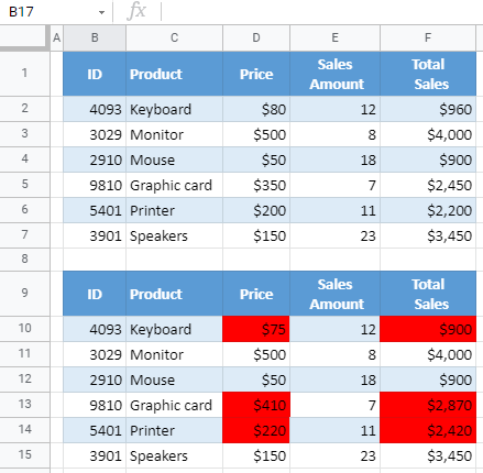
In Excel, you can compare two tables and highlight differences using conditional formatting. Say you have the following two tables with the same structure.

As you can see, there are differences in the two tables (Price and Total Sales for Keyboard, Printer, and Graphic card are changed). Use conditional formatting to highlight these differences in red in the second table.

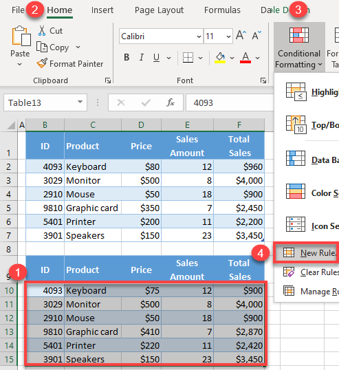
1. Select all cells in the second table (B10:F15) where you want conditional formatting, and in the Ribbon, go to Home > Conditional Formatting > New Rule.

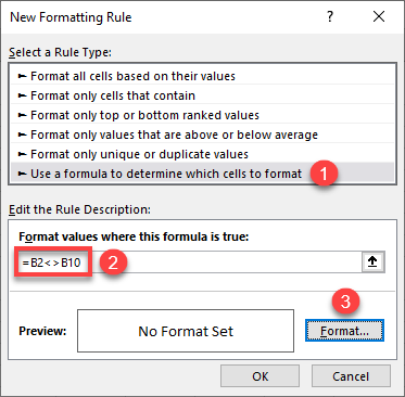
2. In the New Formatting Rule window, choose Use a formula to determine which cells to format for the Rule Type, enter the formula:

=B2<>B10

Then click Format…
This formula goes cell by cell in the selected range. So, in the cell below, it checks whether B3 is different from B11; and in the cell to the right, it checks whether C2 is different from C10; and so on. If the condition is TRUE, the cell is formatted according to the rule.

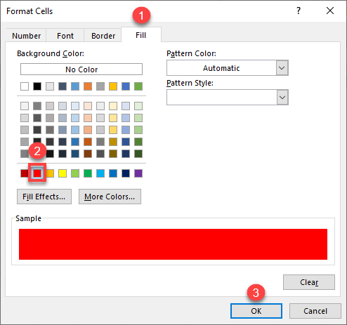
3. In the Format window, go to Fill tab, choose a color (Red), and click OK.

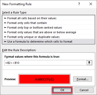
4. Back in the New Formatting Rule window, click OK. Here, you can also see a preview of the formatting to be applied to relevant cells.

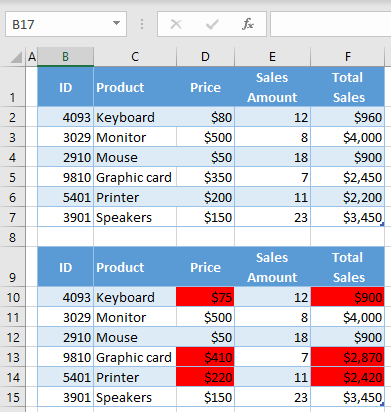
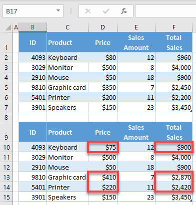
As a result, all differences between the two tables (cells D10, D13, D14, F10, F13, and F14) are highlighted in red in the second table.

See also…

• Using Conditional Formatting with Excel VBA
• How to Compare Two Files for Differences
• How to Compare Two Sheets for Differences
• How to Compare Two Columns for Matches
• How to View Two Sheets From the Same Workbook

Compare Two Tables in Google Sheets

You can do the same comparison in Google Sheets.

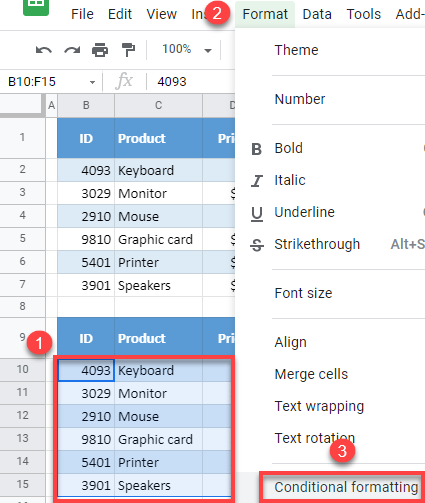
1. Select all cells in the second table (B10:F15) where you want conditional formatting, and in the Ribbon, go to Format > Conditional Formatting .

 

 

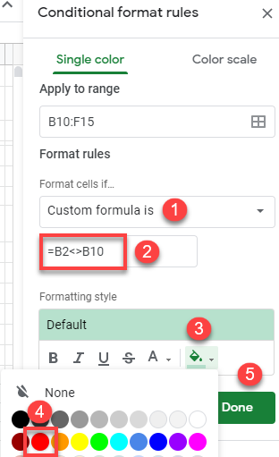
2. In the formatting window on the right side, (1) choose Custom formula is for the rule format, and (2) enter the formula:

=B2<>B10

Click the (3) fill color icon, (4) choose a color (red), and (5) click Done.

 

 

Finally, all differences between the two tables are highlighted in red.