How to Make Negative Numbers Red in Excel & Google Sheets

In this tutorial, you will learn how to format negative numbers with red font in Excel and Google Sheets.

 

 

Make Negative Numbers Red With a Custom Number Format

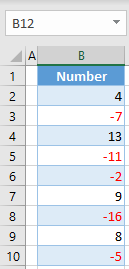
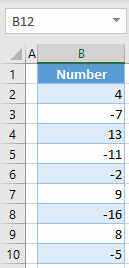
Say you have the list of numbers below in Column B and want to emphasize the negative numbers by making them red.

 

 

The first option to make negative numbers red is to use a custom number format.

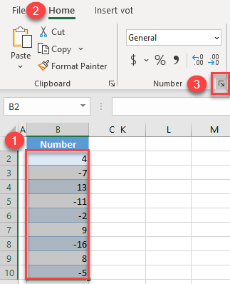
1. Select the range of cells where you want negative numbers to be red and in the Ribbon, go to Home > Number Format (the icon in the bottom right corner of the Number group).

 

 

2. In the Format Cells window, select Custom category, enter #,##0;[Red]-#,##0 for Type, and click OK.

 

 

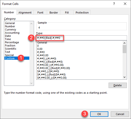
The selected type means that positive numbers will be displayed with default settings, while negative numbers will be red. (The semicolon “;” in the Type box separates positive and negative number formatting.)

As a result, negative numbers in cells B3, B5, B6, B8, and B10, display in red font, as shown below.

 

 

Make Negative Numbers Red With Conditional Formatting

Another option to achieve the same result is to use conditional formatting.

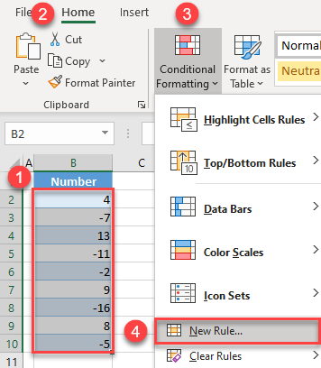
1. Select the range of cells where you want to make negative numbers red and in the Ribbon, go to Home > Conditional Formatting > New Rule…

 

 

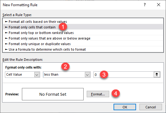
2. In the pop-up window, (1) select Format only cells that contain in Rule type options, (2) choose less than, (3) enter 0 in the Value box, and (4) click Format…

 

 

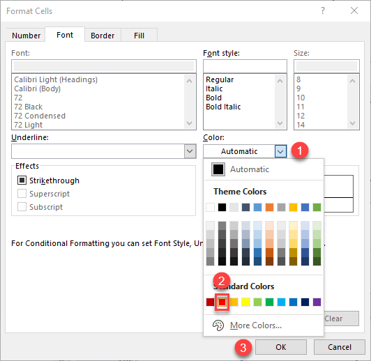
3. In the Font tab of the Format Cells window, click on the Color drop-down menu, choose red as the font color, and click OK.

 

 

4. This takes you back to the New Formatting Rule window. Here you can see the preview of the format and click OK.

 

 

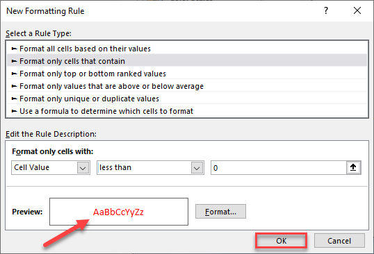
The result is the same as with the method above: All negative values have red font.

 

 

Note: There’s also the option is to use VBA code to format numbers and make negative numbers red.

Make Negative Numbers Red With a Custom Number Format in Google Sheets

You can also format negative numbers with red font in Google Sheets using a custom number format.

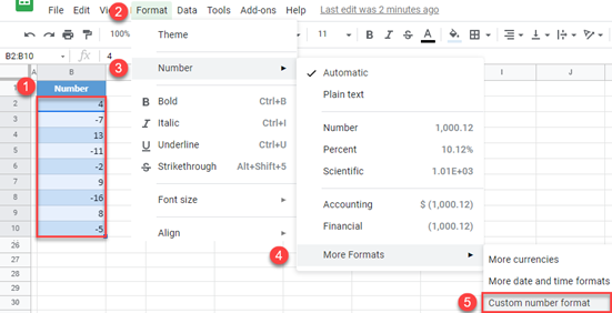
1. Select the range of cells where you want to make negative numbers red and in the Menu, go to Format > Number > More Formats > Custom number format.

 

 

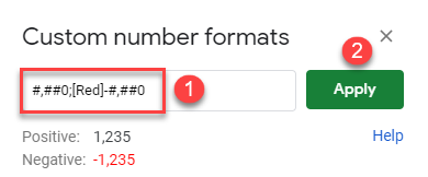
2. In the Custom number formats window, enter the same format used in the Excel example above – #,##0;[Red]-#,##0 – and click Apply.
   In this window, below the input box, you can see a preview of the font.

 

 

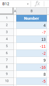
As a result, all negative numbers in the data range are colored in red, as shown below.

 

 

Make Negative Numbers Red With Conditional Formatting in Google Sheets

To do the same thing using Conditional Formatting in Google Sheets, follow these steps:

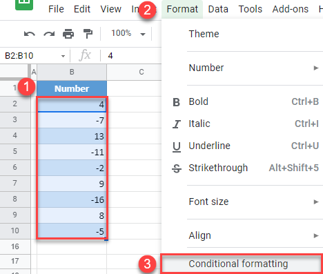
1. Select the range of cells where you want to make negative numbers red and in the Menu, go to Format > Conditional formatting.

 

 

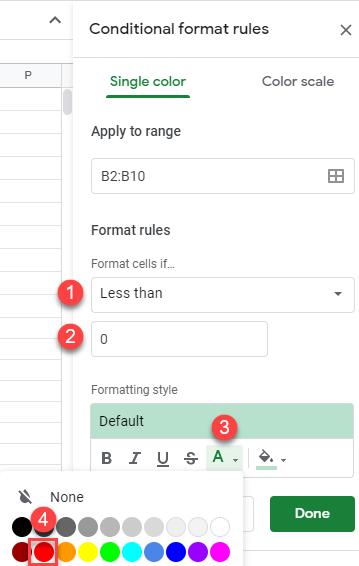
2. In the window on the right side of the sheet, (1) choose Less than in Format rules, and (2) enter 0 in the input box. Under Formatting style, (3) click on the Text Color icon, and (4) choose red.

 

 

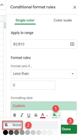
3. Click on the Fill Color icon and choose None, since you don’t need a background fill color. Then click Done.

 

 

Now you’ve created a conditional formatting rule, and all negative values will have red font, as in the previous section.