How to Create a Normal Distribution Bell Curve in Excel

This tutorial will demonstrate how to create a normal distribution bell curve in all versions of Excel: 2007, 2010, 2013, 2016, and 2019.

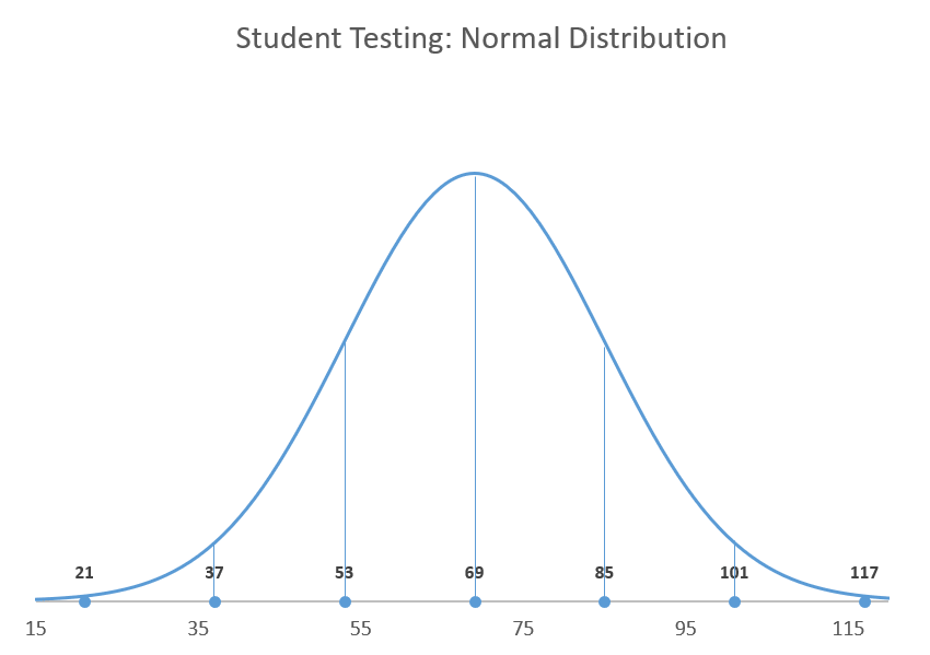
In statistics, a bell curve (also known as a standard normal distribution or Gaussian curve) is a symmetrical graph that illustrates the tendency of data to cluster around a center value, or mean, in a given dataset.

The y-axis represents the relative probability of a given value occurring in the dataset while the x-axis plots the values themselves on the chart to create a bell-shaped curve, hence the name.

The graph helps us analyze whether a particular value is part of the expected variation or is statistically significant and, therefore, has to be examined more closely.

Since Excel doesn’t have any built-in solutions to offer, you will have to plot it yourself. That’s why we developed the Chart Creator Add-in, a tool that allows you to build advanced Excel charts in just a few clicks.

In this step-by-step tutorial, you will learn how to create a normal distribution bell curve in Excel from the ground up:

To plot a Gaussian curve, you need to know two things:

• The mean (also known as the standard measurement). This determines the center of the curve—which, in turn, characterizes the position of the curve.
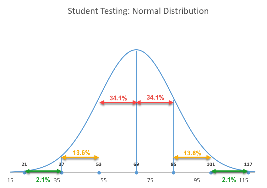
• The standard deviation (SD) of the measurements. This defines the spread of your data in the normal distribution—or in plain English, how wide the curve should be. For instance, in the bell curve shown above, one standard deviation of the mean represents the range between exam scores of 53 and 85.

The lower the SD, the taller the curve and the less your data will be spread out, and vice versa.

It’s worth mentioning the 68-95-99.7 rule that can be applied to any normal distribution curve, meaning roughly 68% of your data is going to be placed within one SD away from the mean, 95% within two SD, and 99.7% within three SD.

Now that you know the essentials, let’s move from theory to practice.

Getting Started

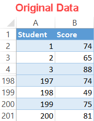
For illustration purposes, let’s assume you have the test scores of 200 students and want to grade them “on a curve,” meaning the students’ grades will be based on their relative performance to the rest of the class:

Step #1: Find the mean.

Typically, you are given the mean and SD values from the start, but if that’s not the case, you can easily compute these values in just a few simple steps. Let’s tackle the mean first.

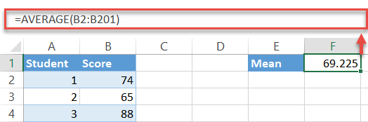
Since the mean indicates the average value of a sample or population of data, you can find your standard measurement using the AVERAGE function.

Type the following formula into any empty cell (F1 in this example) next to your actual data (columns A and B) to calculate the average of the exam scores in the dataset:

=AVERAGE(B2:B201)

 

A quick note: more often than not, you may need to round up the formula output. To do that, simply wrap it in the ROUND function as follows:

=ROUND(AVERAGE(B2:B201),0)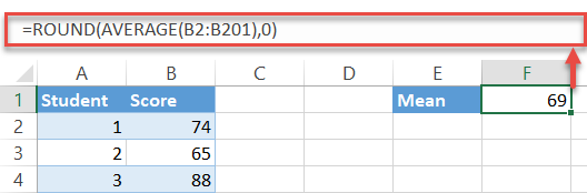

Step #2: Find the standard deviation.

One down, one to go. Fortunately, Excel has a special function to do all the dirty work of finding the standard deviation for you:

=STDEV.P(B2:B201)

Again, the formula picks all the values from the specified cell range (B2:B201) and computes its standard deviation—just don’t forget to round up the output as well.

=ROUND(STDEV.P(B2:B201),0)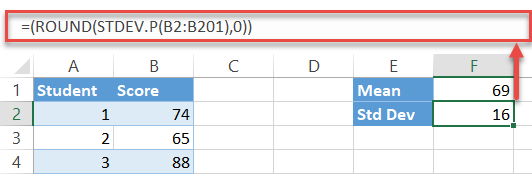

Step #3: Set up the x-axis values for the curve.

Basically, the chart constitutes a massive number of intervals (think of them as steps) joined together with a line to create a smooth curve.

In our case, the x-axis values will be used to illustrate a particular exam score while the y-axis values will tell us the probability of a student getting that score on the exam.

Technically, you can include as many intervals as you want—you can effortlessly erase the redundant data later by modifying the horizontal axis scale. Just make sure you pick a range that will incorporate the three standard deviations.

Let’s start a count at one (as there is no way a student can get a negative exam score) and go all the way up to 150—it doesn’t really matter whether it’s 150 or 1500—to set up another helper table.

1. Pick any empty cell below the chart data (such as E4) and type “1,” the value that defines the first interval.
2. Navigate to the Home tab.
3. In the Editing group, choose “Fill.”
4. Under “Series in,” select “Column.”
5. For “Step value,” type “1.” This value determines the increments that will be automatically added up until Excel reaches the last interval.
6. For “Stop value,” type “150,” the value that stands for the last interval, and click “OK.”

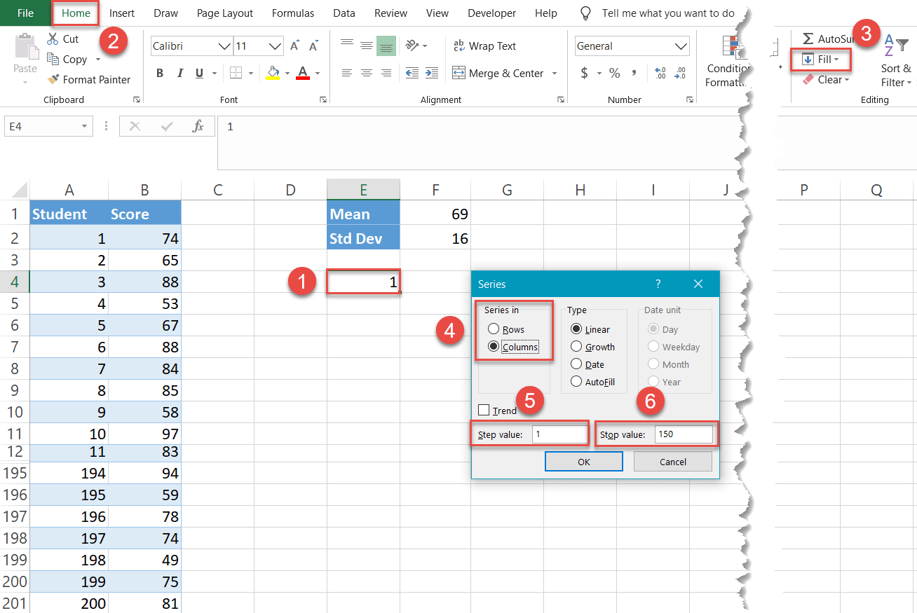
Miraculously, 149 cells in column E (E5:E153) have been filled with the values going from 2 to 150.

NOTE: Do not hide the original data cells as shown on the screenshots. Otherwise, the technique will not work.

Step #4: Compute the normal distribution values for every x-axis value.

Now, find the normal distribution values—the probability of a student getting a certain exam score represented by a particular x-axis value—for each of the intervals. Fortunately for you, Excel has the workhorse to do all these calculations for you: the NORM.DIST function.

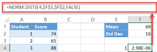
Type the following formula into the cell to the right (F4) of your first interval (E4):

=NORM.DIST(E4,$F$1,$F$2,FALSE)

Here is the decoded version to help you adjust accordingly:

=NORM.DIST([the first interval],[the mean(absolute reference)],[the standard deviation(absolute reference),FALSE)

You lock the mean and SD values so that you can effortlessly execute the formula for the remaining intervals (E5:E153).

Now, double-click on the fill handle to copy the formula into the rest of the cells (F5:F153).

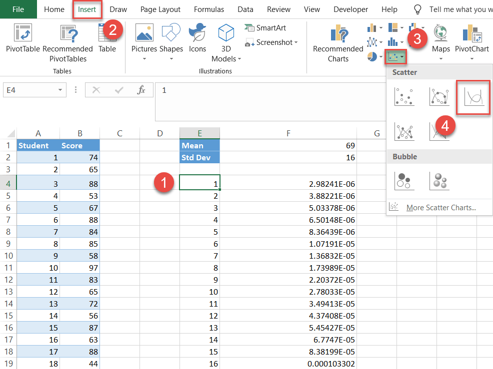
Step #5: Create a scatter plot with smooth lines.

Finally, the time to build the bell curve has come:

1. Select any value in the helper table containing the x- and y-axis values (E4:F153).
2. Go to the Insert tab.
3. Click the “Insert Scatter (X, Y) or Bubble Chart” button.
4. Choose “Scatter with Smooth Lines.”

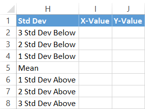
Step #6: Set up the label table.

Technically, you have your bell curve. But it would be hard to read as it lacks any data describing it.

Let’s make the normal distribution more informative by adding the labels illustrating all the standard deviation values below and above the mean (you can also use them for showing the z-scores instead).

For that, set up yet another helper table as follows:

 

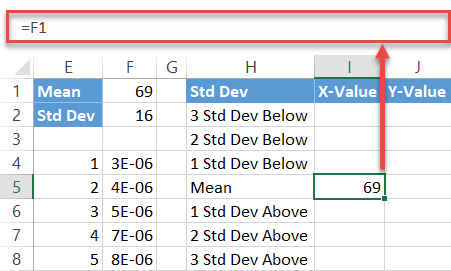
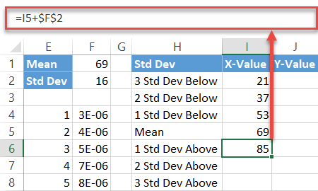
First, copy the Mean value (F1) next to the corresponding cell in column X-Value (I5).

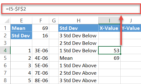
Next, compute the standard deviation values below the mean by entering this simple formula into cell I4:

=I5-$F$2

Simply put, the formula subtracts the sum of the preceding standard deviation values from the mean. Now, drag the fill handle upward to copy the formula into the remaining two cells (I2:I3).

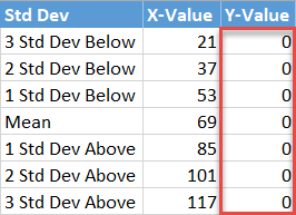
Repeat the same process for the standard deviations above the mean using the mirror formula:

=I5+$F$2

In the same way, execute the formula for the other two cells (I7:I8).

Finally, fill the y-axis label values (J2:J8) with zeros as you want the data markers placed on the horizontal axis.

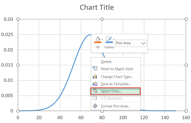
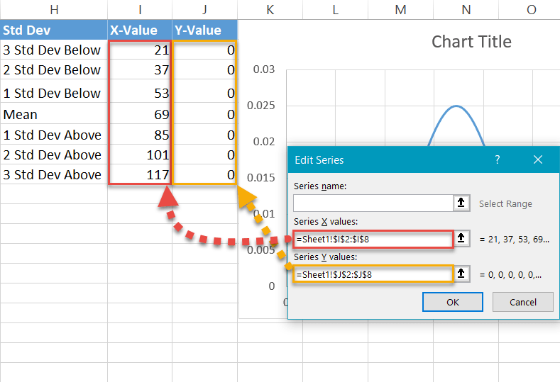
Step #7: Insert the label data into the chart.

Now, add all the data you have prepared. Right-click on the chart plot and choose “Select Data.”

In the dialog box that pops up, select “Add.”

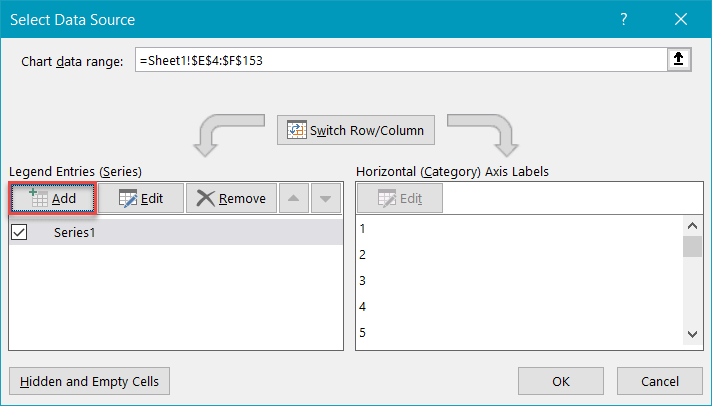
Highlight the respective cells ranges from the helper table—I2:I8 for “Series X values” and J2:J8 for “Series Y values”—and click “OK.”

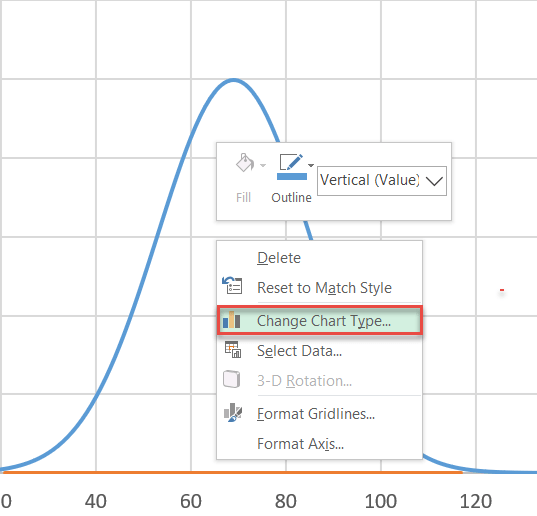
Step #8: Change the chart type of the label series.

Our next step is to change the chart type of the newly-added series to make the data markers appear as dots. To do that, right-click on the chart plot and select “Change Chart Type.”

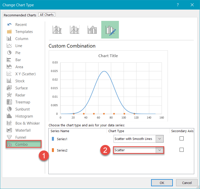
Next, design a combo chart:

1. Navigate to the Combo tab.
2. For Series “Series2,” change “Chart Type” to “Scatter.”
   • Note: Make sure “Series1” remains as “Scatter with Smooth Lines.” Sometimes Excel will change it when you make a Combo Also make sure “Series1” is not pushed to the Secondary Axis—the check box next to the chart type should not be marked.
3. Click “OK.”

Step #9: Modify the horizontal axis scale.

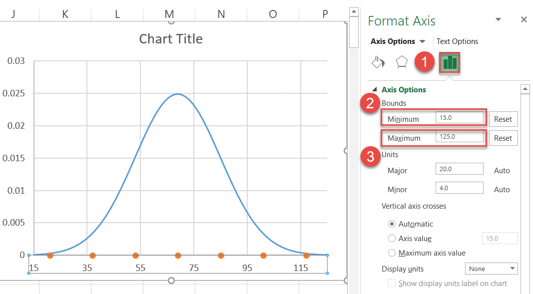
Center the chart on the bell curve by adjusting the horizontal axis scale. Right-click on the horizontal axis and pick “Format Axis” from the menu.

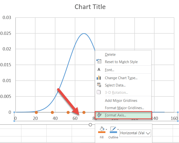
Once the task pane appears, do the following:

• Go to the Axis Options tab.
• Set the Minimum Bounds value to “15.”
• Set the Maximum Bounds value to “125.”

You can tweak the axis scale range however you see fit, but since you know the standard deviation ranges, set the Bounds values a bit away from each of your third standard deviations to show the “tail” of the curve.

Step #10: Insert and position the custom data labels.

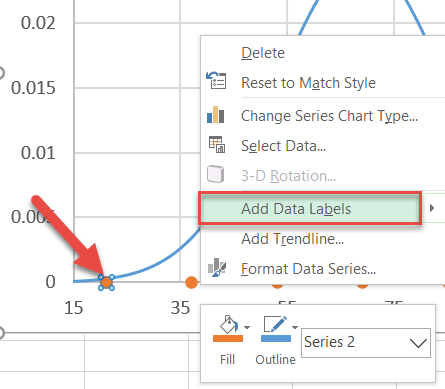
As you polish up your chart, be sure to add the custom data labels. First, right-click on any dot representing Series “Series2” and select “Add Data Labels.”

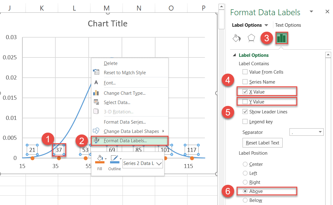
Next, replace the default labels with the ones you previously set up and place them above the data markers.

1. Right-click on any Series “Series2” data label.
2. Select “Format Data Labels.”
3. In the task pane, switch to the Label Options tab.
4. Check the “X Value” box.
5. Uncheck the “Y Value” box.
6. Under “Label Position,” choose “Above.”

Also, you can now remove the gridlines (right-click on them > Delete).

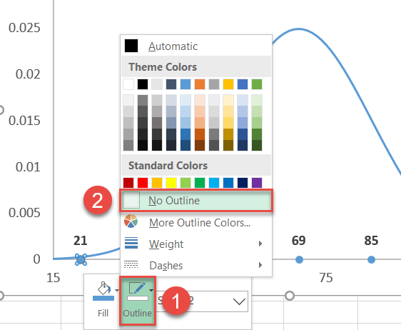
Step #11: Recolor the data markers (optional).

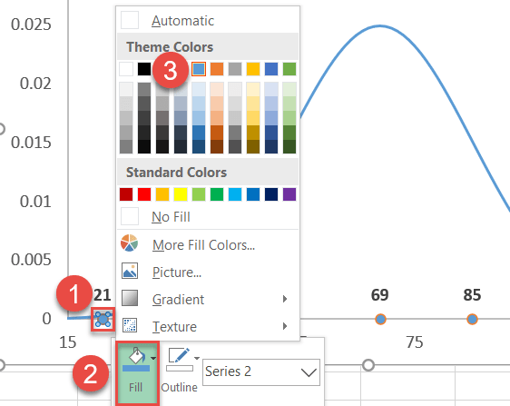
Finally, recolor the dots to help them fit into your chart style.

1. Right-click on any Series “Series2” data label.
2. Click the “Fill” button.
3. Pick your color from the palette that appears.

Also, remove the borders around the dots:

1. Right-click on the same data marker again and select “Outline.”
2. Choose “No Outline.”

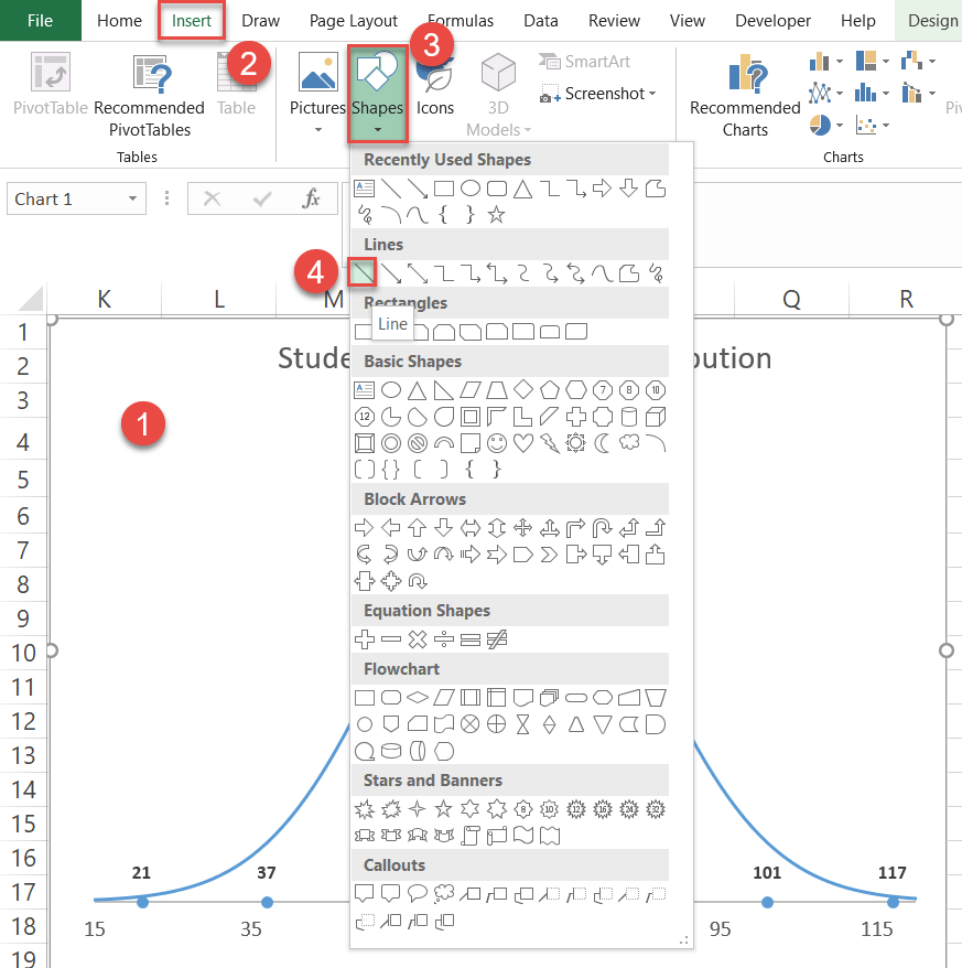
Step #12: Add vertical lines (optional).

As a final adjustment, you can add vertical lines to the chart to help emphasize the SD values.

• Select the chart plot (that way, the lines will be inserted directly into the chart).
• Go to the Insert tab.
• Click the “Shapes” button.
• Choose “Line.”

Hold down the “SHIFT” key while dragging the mouse to draw perfectly vertical lines from each dot to where each line meets the bell curve.

Change the chart title, and your improved bell curve is ready—showing your valuable distribution data.

And that’s how you do it. You can now pick any dataset and create a normal distribution bell curve following these simple steps!