Case Sensitive Lookup – Excel & Google Sheets
Written by
Reviewed by
Download the example workbook
This tutorial will demonstrate how to perform a case-sensitive lookup in Excel using two different methods.
Method 1 – LOOKUP Function
LOOKUP Function
The LOOKUP Function is used to look up an approximate match for a value in a column and returns the corresponding value from another column.
Case-sensitive Lookup
By combining LOOKUP and EXACT, we can create a case-sensitive lookup formula that returns the corresponding value for our case-sensitive lookup. Let’s walk through an example.
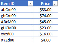
We have a list of items and their corresponding prices (notice that Item ID is case-sensitive unique):
Supposed we are asked to price for an item using its Item ID like so:
![]()
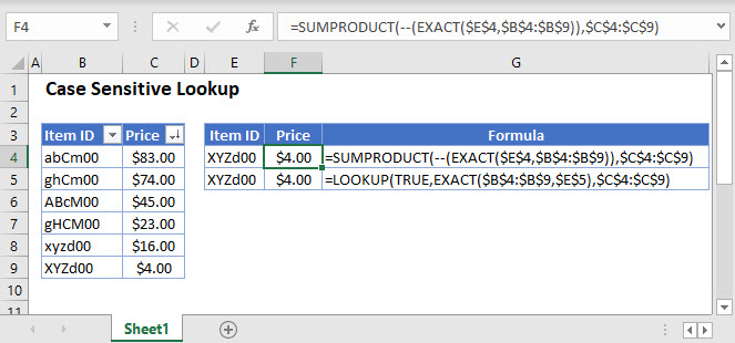
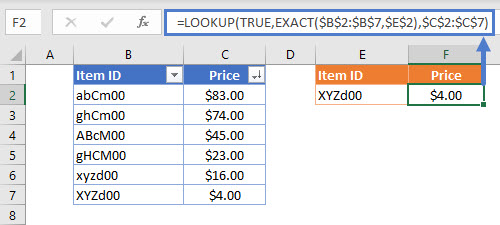
To accomplish this, we can use LOOKUP and EXACT in a formula like so:
=LOOKUP(TRUE,EXACT(<Lookup range>,<lookup value>),<results range>)=LOOKUP(TRUE,EXACT($B$2:$B$7,$E$2),$C$2:$C$7)Limitation: for this method to work, the values must be sorted in descending order
How does the formula work?
The EXACT function checks the Item ID in E2 (lookup value) against the values in B2:B7 (lookup range) and returns TRUE where there is an exact match. Then the LOOKUP function returns the corresponding match in C2:C7 (results range) when the nested EXACT returns TRUE.
Method 2 – SUMPRODUCT Function
SUMPRODUCT Function
The SUMPRODUCT Function is used to multiply arrays of numbers, summing the resultant array.
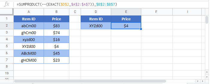
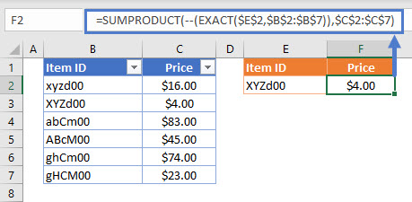
Case-sensitive SUMPRODUCT
Unlike the LOOKUP method, the values do not need to be sorted for this to work. We still need to combine EXACT in a formula to get the results like so:
=SUMPRODUCT(--(EXACT(<lookup value>,<lookup range>)),<results range>)=SUMPRODUCT(--(EXACT($E$2,$B$2:$B$7)),$C$2:$C$7)Limitation: The SUMPRODUCT method will only work when the return value (not the lookup value) is numeric.
How does the formula work?
Like LOOKUP method, the EXACT function deals with finding the case-sensitive match and returns TRUE when there is an exact match or FALSE otherwise. The “–” (known as double unary) converts TRUE to 1 and FALSE to 0. This essentially creates the first array for SUMPRODUCT to multiply with our results array:
{0,1,0,0,0,0}*{16,4,83,45,74,23} = 4Case Sensitive Lookup in Google Sheets
These formulas work exactly the same in Google Sheets as in Excel.