Return Address of Highest Value in Range – Excel & G Sheets

This tutorial will demonstrate how to find and use the cell address of the highest value in a range of cells in Excel and Google Sheets.

Identifying the Highest Value in a Range

First, we will show how find the highest value in a range of cells by using the MAX Function:

This example will identify the highest score in a list:

=MAX(D3:D8)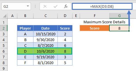

Finding Other Information About the Highest Score

In order to show more information about the highest Score in a list, we can use a combination of the INDEX and MATCH Functions.

The final formula to find the name of the Player with the highest Score is:

=INDEX(B3:B8,MATCH(MAX(D3:D8),D3:D8,0))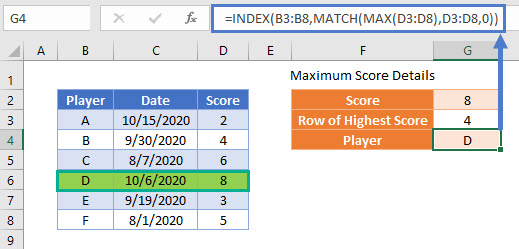

To explain this in steps, we will first identify exactly which cell contains the highest Score in the data range:

=MATCH(MAX(D3:D8),D3:D8,0)

This formula uses the MATCH Function to identify the first cell in the list of Scores that matches the value of the highest Score

=MATCH(8,{2; 4; 6; 8; 3; 5},0)

It finds the first exact match in the 4th cell and so produces the result of 4:

=4

Returning to the complete formula:

=INDEX(B3:B8,MATCH(MAX(D3:D8),D3:D8,0))

We now add the list of Player names and replace the value of the MATCH Formula:

=INDEX({"A"; "B"; "C"; "D"; "E"; "F"}, 4)

Now the INDEX Function returns the cell value of the 4th cell in the list of Player names

="D"

Note that if more than one cell contains a Score of 8, only the first match will be identified by this formula.

Additional information about the data row with the highest Score can be shown by adapting this formula to show values from other columns.

To show the Date of the highest Score, we can write:

=INDEX(C3:C8,MATCH(MAX(D3:D8),D3:D8,0))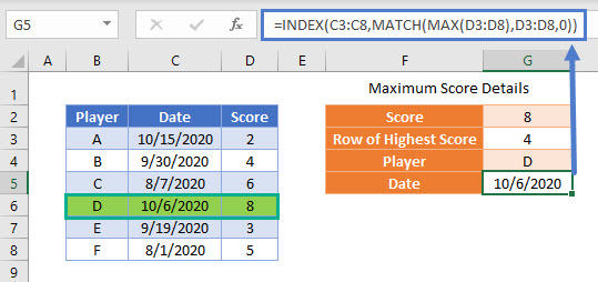

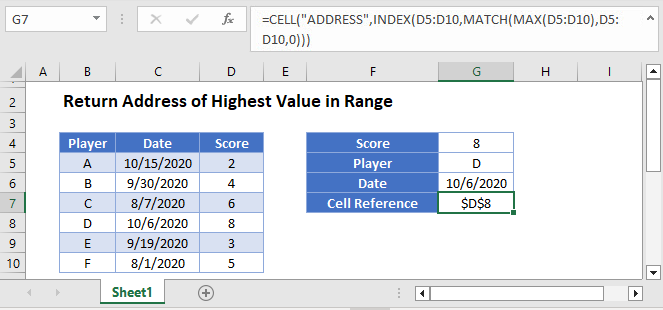
Identifying the Cell Address of the Highest Value in a Range

We can extend the logic of the previous example to show the cell address of the highest Score by using the CELL Function alongside the INDEX, MATCH and MAX Functions that were already used:

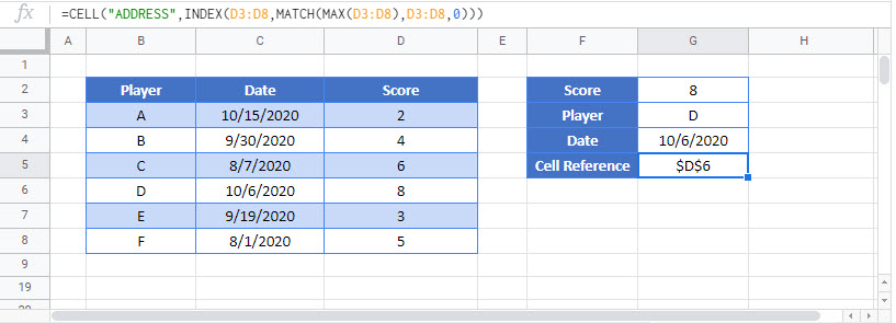
=CELL("ADDRESS",INDEX(D3:D8,MATCH(MAX(D3:D8),D3:D8,0)))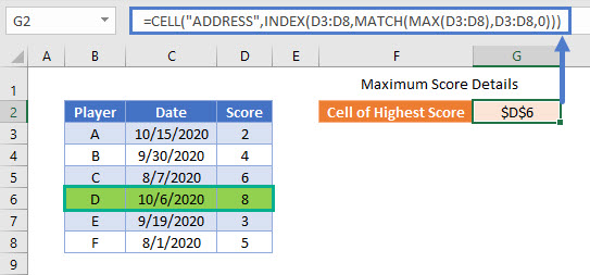

The INDEX and MATCH part of the formula would normally be used to output the value of a cell, but we will use the CELL Function to output a different characteristic. By using the argument “ADDRESS”, and then the previous INDEX–MATCH formula, we can produce a cell reference identifying the highest Score.

This cell reference can then be used as an input in other formulas by using the INDIRECT Function:

=INDIRECT(G2)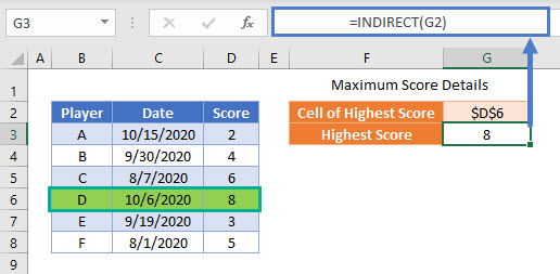

Return Address of Highest Value in Range in Google Sheets

These formulas work exactly the same in Google Sheets as in Excel.