VLOOKUP Function Example
Written by
Reviewed by
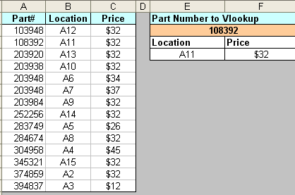
Let’s take a look at the VLOOKUP function. In our example we have a company with a list of part numbers, along with information about them. Let’s asssume this list is very long, and they would like to enter a part# in a cell and have it return information about that part quickly.
This picture shows our desired result. In the orange cell we enter a part number, then the location and price will automagically display

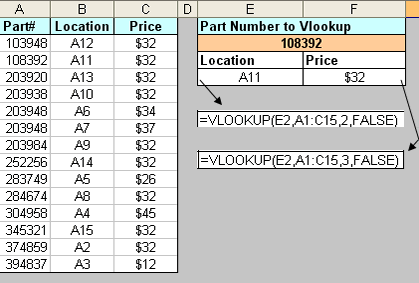
So how do we accomplish this? Here is the VLOOKUP in layman’s syntax
=VLOOKUP(CellToLookup ,RangeToLookIn, WhichColumnToReturn, ExactMatch?)
And now in practice:
1. We need a list of data sorted by the first column.
2. In a blank cell that we would like to return a result from the list, type =VLOOKUP(
3. Click on the cell where we will enter the value to lookup (this will enter the cell in your formula)
4. Hit , (comma)
4. Click and drag to select the entire list including headers
6. Hit, (comma)
7. Type the numerical value of the column you would like to return (A=1, B=2, C=3,,,,)
8. Hit ,(comma)
9. Type “False” and hit enter

Sidenote: Enter “TRUE” to find an approximate match, one reason you might use approximation is on data with Typos or poor standards, for example “MR Man” and it’s actually “MR. Man”.
Sidenote: This works across multiple worksheets. If you would like to store your data in one sheet, and your VLOOKUP in another, it’s the same process.


