Sum Ifs By Week Number – Excel & Google Sheets

This tutorial will demonstrate how to sum data corresponding to specific week numbers in Excel and Google Sheets.

 

Sum If by Week Number

To “sum if” by week number, we will use the SUMIFS Function. But first we need to add a helper column containing the WEEKNUM Function.

The Week Number helper column is calculated using the WEEKNUM Function:

=WEEKNUM(B3,1)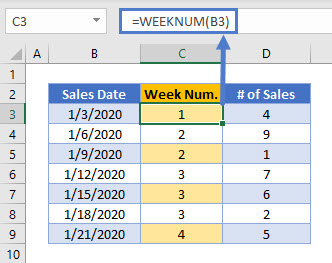

Next, we will use the SUMIFS Function to sum all Sales that take place in a specific Week Number.

=SUMIFS(D3:D9,C3:C9,F3)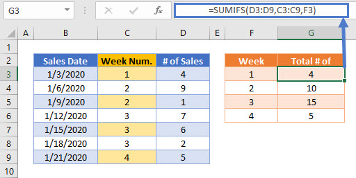

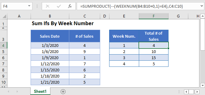
Sum If by Week Number – Without Helper Column

The helper column method is easy to follow, but you can also replicate the calculation in a single formula using the SUMPRODUCT Function in combination with the WEEKNUM Function to sum the Total Number of Sales by Week Number.

=SUMPRODUCT(--(WEEKNUM(B3:B9+0,1)=E3),C3:C9)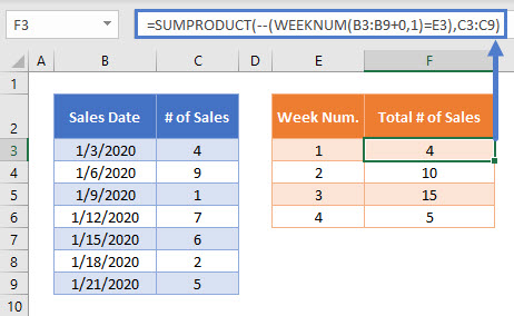

In this example, we can use the SUMPRODUCT Function to perform complicated “sum if” calculations. Let’s walk through the above example.

This is our final formula:

=SUMPRODUCT(--(WEEKNUM(B3:B9+0,1)=E3),C3:C9)

First, the SUMPRODUCT Function lists the array of values from the cell ranges:

=(--(({"1/3/2020"; "1/6/2020"; "1/9/2020"; "1/12/2020"; "1/15/2020"; "1/18/2020"; "1/21/2020"}+0,1)=1), {4; 9; 1; 7; 6; 2; 5})

Then, the WEEKNUM Function calculates the Week Number of each of the Sales Dates.

The WEEKNUM Function is not designed to work with array values, so we must add zero (“+0”) for WEEKNUM to process the values properly.

=SUMPRODUCT(--({1; 2; 2; 3; 3; 3; 4}=1), {4; 9; 1; 7; 6; 2; 5})

Week Number values equal to 1 are changed to TRUE values.

=SUMPRODUCT(--({TRUE; FALSE; FALSE; FALSE; FALSE; FALSE; FALSE}), {4; 9; 1; 7; 6; 2; 5})

Next the double dashes (–) convert the TRUE and FALSE values into 1s and 0s:

=SUMPRODUCT({1; 0; 0; 0; 0; 0; 0}, {4; 9; 1; 7; 6; 2; 5})

The SUMPRODUCT Function then multiplies each pair of entries in the arrays to produce an array of Number of Sales that have a Week Number of 1:

=SUMPRODUCT({4; 0; 0; 0; 0; 0; 0})

Finally, the numbers in the array are summed together:

=4

This formula is then repeated for the other possible values of Week Number.

More details about using Boolean statements and the “–” command in a SUMPRODUCT Function can be found here.

Locking Cell References

To make our formulas easier to read, we’ve shown the formulas without locked cell references:

=SUMPRODUCT(--(WEEKNUM(B3:B9+0,1)=E3),C3:C9)

But these formulas will not work properly when copy and pasted elsewhere in your file. Instead, you should use locked cell references like this:

=SUMPRODUCT(--(WEEKNUM($B$3:$B$9+0,1)=E3),$C$3:$C$9)

Read our article on Locking Cell References to learn more.

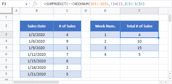
Sum If by Week Number in Google Sheets

These formulas work exactly the same in Google Sheets as in Excel.

However, the WEEKNUM Function is more flexible in Google Sheets than in Excel, and accepts array inputs and outputs. Therefore the {Array}+0 operation in the WEEKNUM(B3:B9+0,1) formula is not required.

The full SUMPRODUCT formula can be written in Google Sheets as:

=SUMPRODUCT(--(WEEKNUM($B$3:$B$9,1)=E3),$C$3:$C$9)