CUMPRINC Function Examples – Excel, VBA, & Google Sheets

This tutorial demonstrates how to use the Excel CUMPRINC Function in Excel to calculate the cumulative principal amount paid on a loan.

CUMPRINC Function Overview

The CUMPRINC Function Calculates the payment amount.

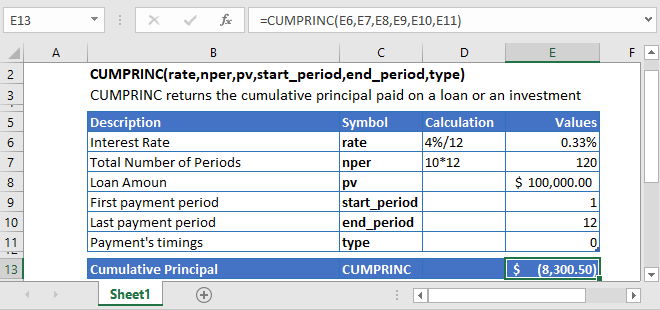
To use the CUMPRINC Excel Worksheet Function, select a cell and type:

 

 

(Notice how the formula inputs appear)

CUMPRINC Function Syntax and Inputs:

=CUMPRINC(rate,nper,pv,start_period,end_period,type)

rate – The interest rate for each period.

nper – The total number of payment periods.

pv – The present value of the loan or investment.

start_period – The number of the first period over which the cumulative principal amount is to be calculated. Its value must be an integer and between 1 and nper.

end_period – The number of the last period over which the cumulative principal amount is to be calculated.

type – The payment type. 1 for the beginning of the period. 0 for the end of the period (default if omitted).

 

What is the Excel CUMPRINC Function?

The Excel CUMPRINC function is a financial function and returns the cumulative principal payment paid on a loan or an investment between two specified periods. For this function, the interest rate and the payment schedule must be constant.

Calculate Cumulative Principal Payment of a loan

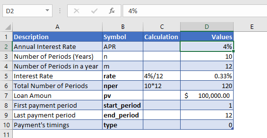
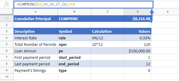
Let’s use the Excel CUMPRINC function to calculate the cumulative principal amount paid, during the first year of a loan of $100,000. And this loan has to be paid off completely in 10 years with a 4% annual interest rate. The monthly payment of the loan has to be calculated.

As the payments are made monthly, the annual interest rate is converted into monthly interest by

Monthly Interest Rate – 4% (annual interest rate) / 12 (months per year) = 0.33%

and the number of payments per period is converted into the monthly number of payments by

NPER – 10 (years) * 12 (months per year) = 120

And the cumulative principal amount is to be determined on its first year, so the starting period and end period values are:

start_period = 1

end_period = 12

The Formula used for the calculation of cumulative principal payment is:

=CUMPRINC(D7,D8,D9,D10,D11,D12)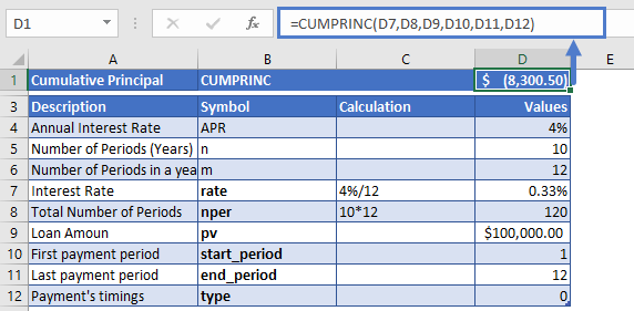

The cumulative principal amount paid during the first year of the loan is

CUMPRINC = -$8,300.50

The result of the CUMPRINC function is a negative value since the principal amount paid is outgoing cash flow.

Calculate Cumulative Principal Payment during 4th year of a loan

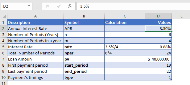
Suppose a student loan has taken out a loan of  $40,000 with an annual interest of 3.5%. The loan time period is 6 years and the payments are being made at the start of every quarter. We need to calculate the cumulative principal amount paid during the 4th year of the loan.

The payments are made monthly, so the annual interest rate is converted into monthly interest by

Monthly Interest Rate – 3.5% (annual interest rate) / 4 (quarters per year) = 0.25%

and the number of payments per period is converted into the monthly number of payments by

NPER – 6 (years) * 4 (quarters per year) = 24

And the cumulative principal amount is to be determined for its 4th year, so the starting period and end period values are:

start_period = 19

end_period = 22

The Formula used for the calculation is:

=CUMPRINC(D7,D8,D9,D10,D11,D12)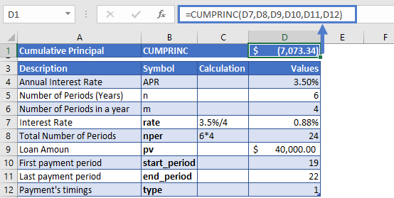

The cumulative principal amount paid during the 4th year is

CUMPRINC= -$7,073.34

The result of the CUMPRINC function is a negative value since the principal amount paid is outgoing cash flow.

Additional Notes

Make sure the units of nper and rate are consistent, i.e. in case of monthly interest rate the number of periods of investment should also be in months.

In the Excel Financial Functions the cash outflows, such as deposits, are represented by negative numbers and the cash inflows, such as dividends, are represented by positive numbers.

#NUM! Error occurs if the values of rate, nper, pv are less than and equal to zero; the values of start_period and end_period are less than or equal to zero, and also greater than nper; the start_period > end_period; or the value of the type argument is other than 0 or 1.

#VALUE! Error occurs if any of the arguments’ value is non-numeric.

Return to the List of all Functions in Excel

 

CUMPRINC in Google Sheets

All of the above examples work exactly the same in Google Sheets as in Excel.

CUMPRINC Examples in VBA

You can also use the CUMPRINC function in VBA. Type:

application.worksheetfunction.cumprinc(Rate,Nper,Pv,StartPeriod,EndPeriod,Type)

For the function arguments (Rate, etc.), you can either enter them directly into the function or define variables to use instead.