MIRR Function Examples – Excel, VBA, & Google Sheets

This tutorial demonstrates how to use the Excel MIRR Function in Excel to calculate the modified internal rate of return.

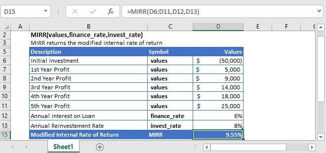
MIRR Function Overview

The MIRR Function Calculates the rate of return.

To use the MIRR Excel Worksheet Function, select a cell and type:

 

 

(Notice how the formula inputs appear)

MIRR Function Syntax and Inputs:

=MIRR(values,finance_rate,invest_rate)

values– The values argument consists of an array or a reference to a range of cells representing the series of cash flows. And the values argument must contain at least one negative and one positive value for the calculation.

finance_rate – It’s the cost of borrowing (in case of negative cash flows) or the interest rate paid to finance the investment.

invest_rate – It’s the rate of return earned from reinvesting the cash flows.

 

What Is MIRR?

The Modified Internal Rate of Return (MIRR) is used to measure the attractiveness of an investment. It’s used to rank the same size of alternate investments.

The MIRR is a modification of the simple Internal Rate of Return. The modified internal rate of return (MIRR) assumes that the interest received on the reinvestment to be different. While the simple IRR assumes the cash flows is reinvested at IRR itself.

MIRR is calculated using the following equation.

Where:

n = number of equal periods at the end of which the cash flows occur (not the number of cash flows)

PV = Present Value (at the beginning of the first period)

FV = Future Value (at the end of the last period)

What is the Excel MIRR Function?

The Excel MIRR function calculates the Modified Internal Rate of Return for a series of cash flows occurring at regular intervals.

The Excel MIRR function uses the following formula to calculate the MIRR:

Where:

n = number of time periods

rrate = invest_rate

frate = finance_rate

NPV = Net Present Value

Calculate the Modified Internal Rate of Return on a buisness

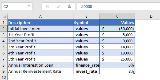
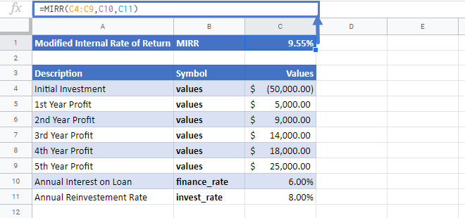
Consider you took out a loan of $50,000 and started a business. The interest paid on this loan is 6% yearly. The net profit generated from the business for the first five years is given in the above table. These net profits were reinvested in the business at an annual rate of 8%.

Here, the initial investment is a negative value as it shows an outgoing payment, and the net profits are represented by positive values.

Initial investment = -$50,000

The formula used to calculate the modified internal rate of return is:

=MIRR(C4:C9,C10,C11)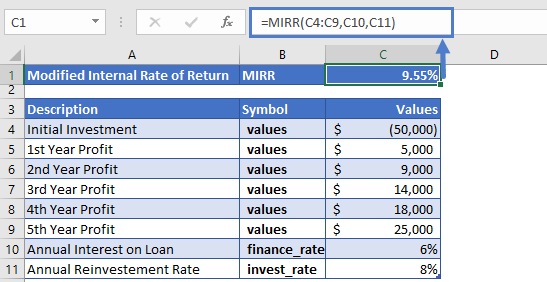

The Modified Internal Rate of Return calculated through Excel MIRR function is

MIRR = 9.15%

Calculate the Modified Internal Rate of Return on an investment

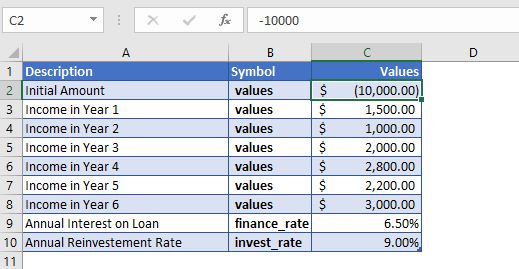
Suppose you invested $10,000 in a fund and this money was borrowed at a rate of 6.5%. The net income cash flows you get are given in the above table. The rate of interest you get from your reinvested capital is 9%.

The formula used to calculate the modified internal rate of return is:

=MIRR(C4:C10,C11,C12)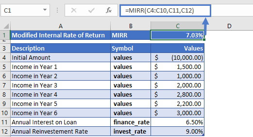

The Modified Internal Rate of Return (MIRR) we get after 6 years is

MIRR = 7.03%

 

Additional Notes

The values should in chronological order, meaning the sequence of payments and income should be entered correctly.

#DIV/0! Error occurs if the values argument doesn’t contain at least one negative and one positive value.

#VALUE! Error occurs when the supplied arguments are non-numeric.

Return to the List of all Functions in Excel

 

MIRR in Google Sheets

All of the above examples work exactly the same in Google Sheets as in Excel.

MIRR Examples in VBA

You can also use the MIRR function in VBA. Type:

application.worksheetfunction.mirr(ValueArray,FinanceRate,ReinvestRate)

For the function arguments (FinanceRate, etc.), you can either enter them directly into the function or define variables to use instead.