PERCENTRANK Function Examples – Excel & Google Sheets

This tutorial demonstrates how to use the PERCENTRANK Function in Excel to calculate the rank of a value in a data set as a percentage of the data set.

What Is the PERCENTRANK Function?

The PERCENTRANK Function returns the percentage rank of a value in a given range of data, inclusive of the first and last values.

PERCENTRANK Is a “Compatibility” Function

As of Excel 2010, Microsoft replaced PERCENTRANK with two variations: PERCENTRANK.INC (which is the same as PERCENTRANK) and PERCENTRANK.EXC (which returns the percent rank exclusive of the first and last values).

PERCENTRANK still works, so older spreadsheets using it will continue to function as normal. However, Microsoft may discontinue the function at some point in the future, so unless you need to retain compatibility with older versions of Excel, you should use PERCENTRANK.INC or PERCENTRANK.EXC.

How to Use the PERCENTRANK Function

Use PERCENTRANK like this:

=PERCENTRANK(C4:C13,F3,3)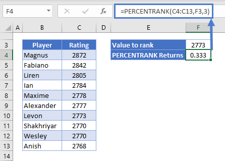

The table shows the ratings of a group of chess players. PERCENTRANK can tell us what percentage of the scores in this group are below a given value.

Here’s how it works:

• The first argument, C4:C13, is the data range
• The second argument is the value that we want to rank
• The third argument is called “significance”, and it’s simply the number of decimal places we want in the result

So, we’ve asked PERCENTRANK what percentage of scores in this group are lower than 2773, and we want the answer to 3 decimal places.

Since the value of 2773 actually appears in our data range, the calculation is fairly straightforward. Excel calculates it as follows:

Percent Rank = Number of values below / (Number of values below + number of values above)

Plugging our numbers in:

Percent Rank = 3 / (3 + 6) = 0.333 (or 33.333%)

When Values Don’t Appear in the Data Range

What about if we ask for the percent rank of a value that doesn’t appear in the dataset?

In such cases, PERCENTRANK first calculates the percent ranks of the two values it lies between, and then calculates an intermediate value.

Here’s an example:

=PERCENTRANK(C4:C13,F3,3)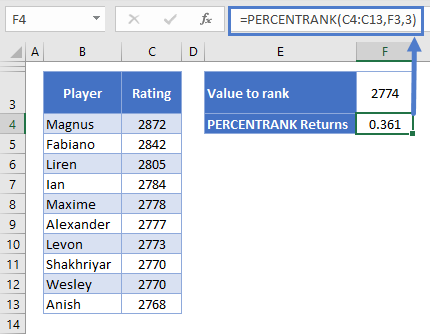

Now we want the percent rank of 2774, and we get 0.361, or 36.1%.

Why? 2774 sits between Levon’s score of 2773 and Alexander’s score of 2774. In fact, it’s 25% of the way between the two scores, so the percent rank returned is 25% of the distance between the two scores’ percent ranks.

The calculation works like this:

Lower percent rank + (distance*(Higher percent rank – lower percent rank))

We already know Levon’s percent rank is 0.333. Alexander’s is 0.444, so plugging these in:

0.333 + (0.25 * (0.444 – 0.333)) = 0.36075

Since we’ve set our significance to 3 in the above formula, that rounds to 0.361.

PERCENTRANK.INC

As noted earlier, Microsoft has replaced the PERCENTRANK function, so you should try not to use it wherever possible.

One of its replacements, PERCENTRANK.INC, works in exactly the same way:

=PERCENTRANK.INC(C4:C13,F3,3)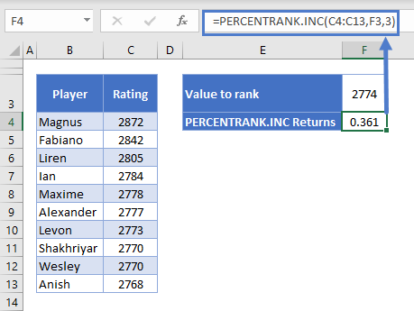

You define the same arguments in PERCENTRANK.INC that we just saw in PERCENTRANK:

• the data range
• the value you want to rank
• and the significance.

As you can see here, it returns the same result.

The “INC” part of the function’s name is short for “inclusive”. It means that the function sets the largest value in the set to 100%, the smallest to 0%, and then positions the rest of the scores at intermediate percentages between the two.

These intermediate percentages are determined with the calculation:

1 / (n – 1)

Where n is the number of data points in the range.

Since we have 10 data points, that works out to 1 / (10 – 1) = 0.111 or 11%.

So the lowest score’s percent rank is 0, the next one is 11%, then 22%… and so on all the way to 100%.

PERCENTRANK.EXC

PERCENTRANK.EXC is very similar, and you use it in the same way, but it calculates the results a little differently.

Use it like this:

=PERCENTRANK.EXC(C4:C13,F3,3)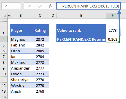

We want the percent rank of 2773, Levon’s score again, but this time we get 0.363, or 36.3% instead of the 33% we saw earlier.

Why is that?

Well the “EXC” is short for “Exclusive”, meaning PERCENTRANK.EXC excludes the first and last values when calculating the percentage difference between each score.

The distances between each score are calculated as follows:

1 / (n + 1)

Since we have 10 data points, this works out to 1 / (10 + 1) = 0.0909, just over 9%.

So with PERCENTRANK.EXC, the lowest score’s percent rank is 9%, the next 18%, and so on up to 100%.

Now we can see where the difference comes from – Levon’s score is the fourth highest, so his percent rank is:

0.0909 * 4 = 0.363

Everything else works the same way, including the equation for calculating the percent rank of score that don’t appear in the data set – Excel just uses these 9.09% intervals instead of the 11.111% intervals we saw with PERCENTRANK.INC.

 

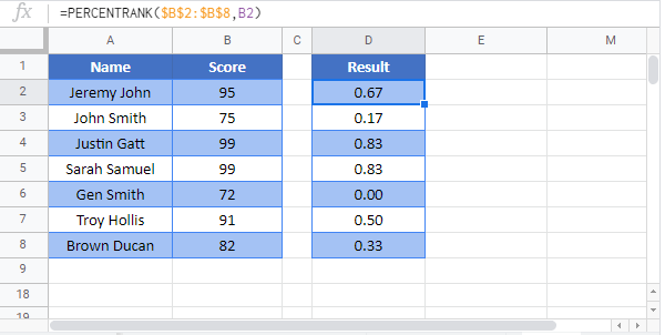
PERCENTRANK Function in Google Sheets

The PERCENTRANK  Function works exactly the same in Google Sheets as in Excel: