How Does the SPARKLINE Function Work in Google Sheets?

This tutorial demonstrates how the SPARKLINE Function works in Google Sheets.

SPARKLINE Function Overview

A sparkline is a miniature chart within a single cell. In Google Sheets, you need a formula to insert sparklines into your worksheet. To use the SPARKLINE Function, select the relevant cell and type:

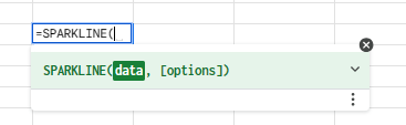
If the syntax is not showing, click on the small ? to the left of the function.

data – This needs to be populated with the range of cells that contain the data for the sparkline.

[options] – Customize options such as the color and type of sparkline. Square brackets indicate that this input isn’t mandatory; only the data is necessary.

Insert a Basic Sparkline

Consider the following data:

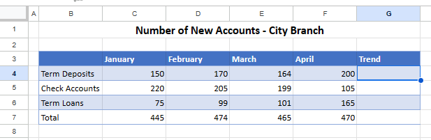
Cells C4 to F4 contain a dataset with trends for several accounts across four calendar months.

▸ To create a basic sparkline, type in the formula shown below into G4.

=SPARKLINE(C4: F4)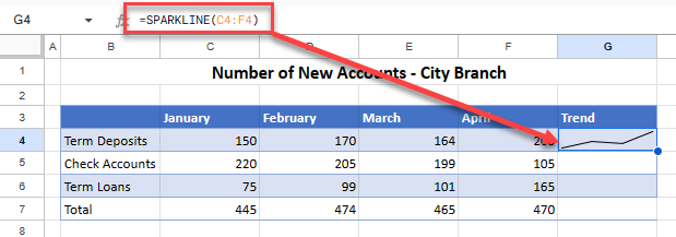

A visualization of the data in C4 to F4 is then displayed in cell G4.

Sparkline Options

The SPARKLINE Function is divided into data and options sections. In the options section, you can set different types of sparklines as well as an array of options to customize the sparkline.

Types of Sparklines

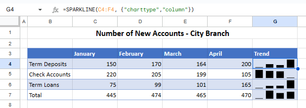
You can have one of four different chart types for the sparkline: column, line, bar, or win/loss. The default sparkline is a line chart. A win/loss chart is a special type of column chart that plots positive and negative outcomes.

▸ To create a bar sparkline, add bar as a SPARKLINE formula input. (The charttype section has to be enclosed in curly brackets to work correctly.)

=SPARKLINE(C4:F4,{"charttype","bar"})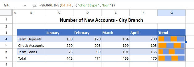

Replace the word bar with column or winloss to create different types of sparklines.

Line Width (Line Sparklines)

Change the width of the line for a Line sparkline with the linewidth input. Column G in the picture below illustrates four different possible weights.

=SPARKLINE(C4:F4,{"linewidth",7})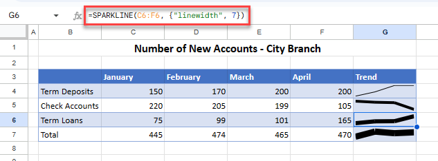

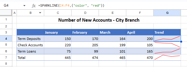
Color

To change the color of the default sparkline, add a color input to the formula.

=SPARKLINE(C4:F4, {"color","red"})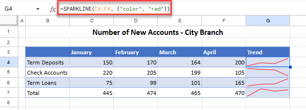

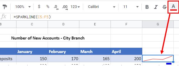
Define Color

Colors can be written using their names or their hex code. For example, the formula below also returns a red sparkline:

=SPARKLINE(C5:F5,{"color","#FF0000"})

You can also change the color of the sparkline by changing the color of the text in the cell selected. In the Menu, click Text Color and choose a color.

Multiple Inputs

To change both the color and type of a sparkline, combine the two options in one formula, separating them with a semicolon. Read on for some examples.

Column Sparkline With Custom Colors

The picture below shows three color settings in Column G.

=SPARKLINE(C6:F6, {"color","blue"; "charttype", "column"})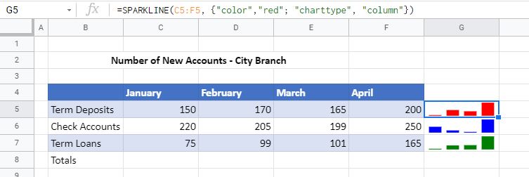

Multiple Colors in One Column Sparkline

Set the color of the column with the lowest value, or the column with the highest value using lowcolor and highcolor.

=SPARKLINE(C4:F4,{"charttype","column";"color","red","lowcolor","blue","highcolor","green"})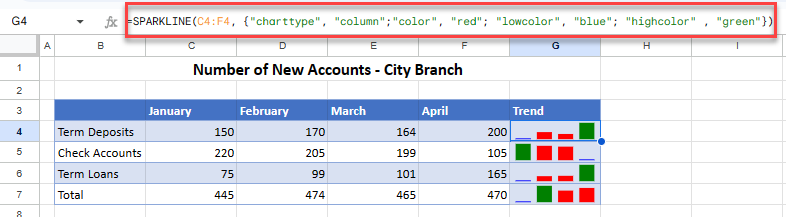

Use firstcolor or lastcolor to set the colors of the first and last columns.

=SPARKLINE(C4:F4, {"charttype", "column"; "color", "red", "firstcolor", "blue", "lastcolor", "green"})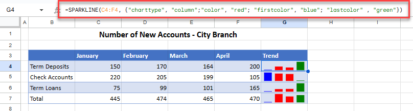

If one of the columns of data has a negative number and you want negative columns in a different color, use negcolor.

=SPARKLINE(C4:F4, {"charttype", "column"; "color", "red", "firstcolor", "blue", "lastcolor", "green", "negcolor", "yellow"})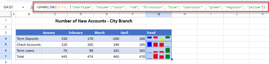

Bar Sparkline With Alternating Colors

With a bar sparkline, you can set alternating colors using color1 and color2.

=SPARKLINE(C4:F4, {"charttype", "bar"; "color1", "blue", "color2", "green"})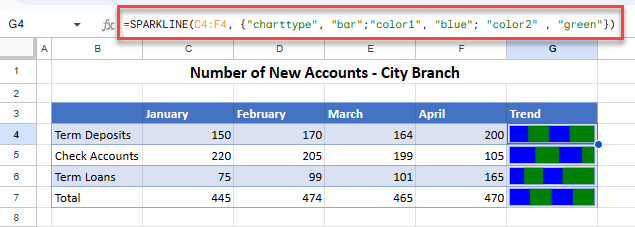

Min / Max Values and Alignment (Bar Sparkline)

If you add the max input to your bar sparkline, the cell that the sparkline is in fills to the total for that the data. In the example below, set the max value to 1000 whereas if you add up the values from C4:F4 you get a total of 720. The sparkline therefore fills up 72% of the cell in which it is situated.

=SPARKLINE(C4:F4, {"charttype", "bar"; "max", 1000})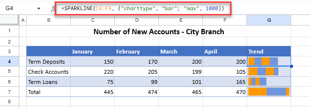

If you use the max input, you may also want to set the alignment to the left or right of the cell using the rtl input.

=SPARKLINE(C4:F4,{"charttype","rtl",true,"bar";"max",1000})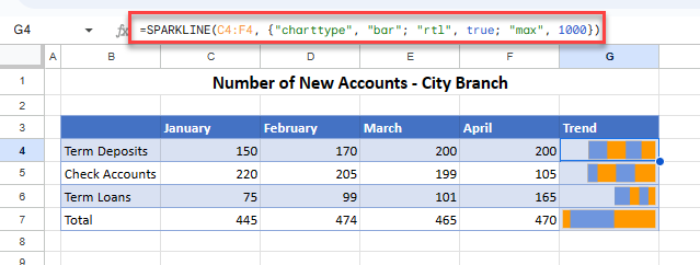

Other Options

• xmin and xmax – Set minimum and maximum values along the horizontal axis (line sparklines only).
• ymin and ymax – Set minimum and maximum values along the vertical axis (line and column sparklines only).
• empty – Decide how empty cells are treated – this can be set to zero or ignore.
• nan – Decide how cells with non-numeric data are treated; this can be set to convert or ignore.
• linewidth – Set the thickness of the line. The higher the line width value, the thicker the line (line sparklines only).
• negcolor – Set the color for negative columns (column and win/loss sparklines only)
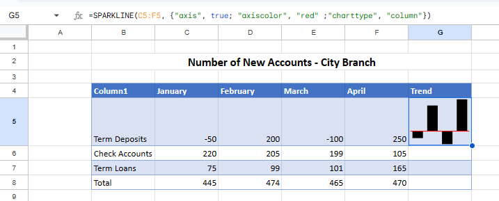
• axis – Determine whether an axis must be drawn and can be set to true or false (column and win/loss sparklines only. Axes are visible if a sparkline chart contains both negative and positive values).

Note: All inputs above – excluding true/false – must be in double quotes in the formula.