How to Hide Rows Based on Cell Value in Excel & Google Sheets

This tutorial demonstrates how to hide rows based on values they contain in Excel and Google Sheets.

 

 

Hide Rows Based on the Value of a Cell

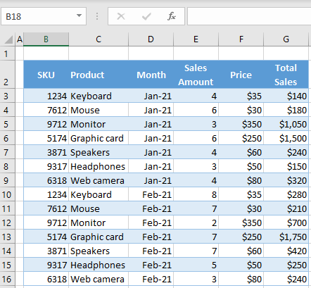
In Excel, you can use filters to hide rows in a table. To exclude cells with certain values, set an appropriate filter. To see how this works, let’s start with the data range pictured below:

 

 

Hide Cells Less Than

To hide rows in this table with Total Sales (Column G) less than $400, filter Column G and display values greater than 400.

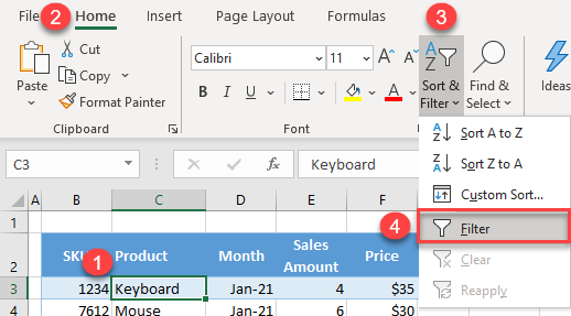
1. First, turn on filtering. Click on any cell in the data range (B2:G16) and in the Ribbon, go to Home > Sort & Filter > Filter.

 

 

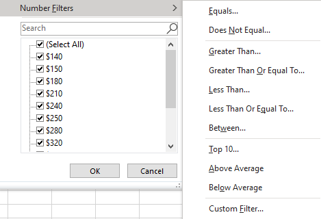
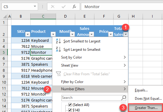
2. Click on the filter button next to Total Sales (cell G2), go to Number Filters, and choose Greater Than…

 

 

3. In the filter pop-up window, enter 400 and click OK.

 

 

As a result, rows with values less than 400 in Column G are hidden.

 

 

Hide Cells Equal To

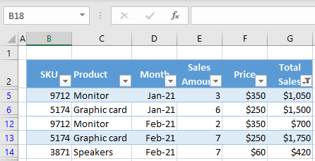
Now let’s use the initial data range (with all filters cleared) to hide rows with the SKU (Column B) 1234. Use a number filter again to filter and display values in Column B that don’t equal 1234.

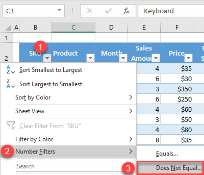
1. Click on the filter button next to SKU (cell B2), go to Number Filters, and choose Does Not Equal…

 

 

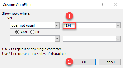
2. In the pop-up window, enter 1234 and click OK.

 

 

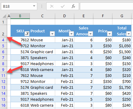
Now, rows with the SKU 1234 (3 and 10) are hidden while all other rows are displayed.

 

 

Hide a Number of Rows Based on Values

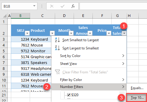
You can also filter the top n rows by Total Sales (Column G) and hide all rows with total sales not in the top 5. Go back to the initial, unfiltered data range and follow these steps:

1. Click on the filter button next to Total Sales (cell G2), go to Number Filters, and choose Top 10…

 

 

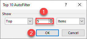
2. In the pop-up window, enter 10, and click OK.

 

 

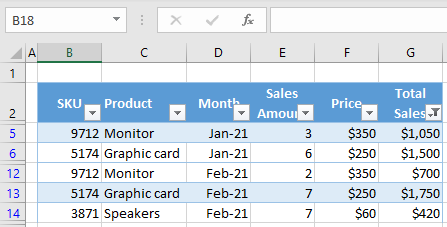
Now, the rows with the top 5 values of total sales are displayed, and all rows where values are not in the top 5 are hidden.

 

 

Other options for number filters include:

• equals,
• less than / less than or equal to,
• between,
• below/above average, and
• custom filter.

Note: You can also use VBA code to filter numbers and hide rows based on a cell value.

Hide Rows Based on Value in Google Sheets

You can hide rows based on cell value in Google Sheets in almost the same way. Let’s use the same example to filter Total Sales (Column G) and display values greater than $400. Doing this hides rows where the total sales value is less than $400.

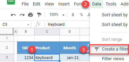
1. To create a filter, click anywhere in the data range (B2:G16) and in the Menu, go to Data > Create a filter.

 

 

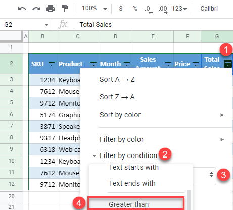
2. Click on the filter button next to Total Sales (cell G2) and go to Filter by condition. In the drop-down list, choose Greater than.

 

 

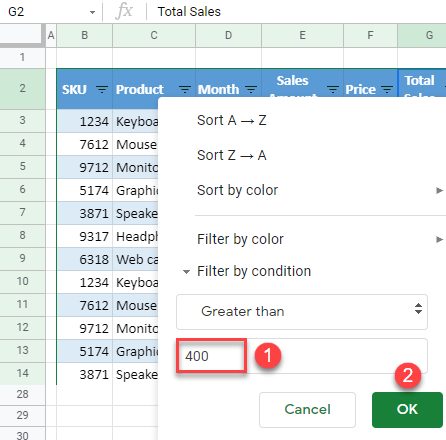
3. Enter 400 in the text box and click OK.

 

 

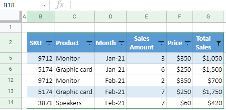
As a result, rows with total sales less than $400 are hidden; only those with a value greater than $400 are displayed.

 

 

Like Excel, Google Sheets has more options to filter by number:

• is equal to / not equal to,
• greater than or equal to,
• less than / less than or equal to,
• is between / is not between, and
• custom formula.